Latent Mobility Infections

Code

import numpyro

numpyro.enable_x64()

import jax.numpy as jnp
import jax.random as random
import numpy as np
from numpyro.infer import Predictive
import pandas as pd
import plotnine as p9
import warnings
from plotnine.exceptions import PlotnineWarning

warnings.filterwarnings("ignore", category=PlotnineWarning)

from _tutorial_theme import theme_tutorial

Code

from pyrenew.latent import MobilitySubpopulationInfections, RandomWalk
from pyrenew.deterministic import DeterministicPMF, DeterministicVariable

Overview

SubpopulationInfections gives each subpopulation its own renewal equation, and infections in one subpopulation do not depend on infections in any other. MobilitySubpopulationInfections keeps the same \(\mathcal{R}(t)\) structure, a shared baseline plus deviations that sum to zero, but treats subpopulations as home regions whose residents spend part of each day in other regions. Infections among residents of a region then depend on transmission in the regions they visit and on the infectious visitors their own region receives.

The class implements Equation 2 of Roy, Clapham, and Mishra (2025), Incorporating human mobility to enhance epidemic response and estimate real-time reproduction numbers. For home region \(i\) on day \(t\):

\[ I_{t,i} = \sum_{j=1}^{n} \frac{m_{ji}\, S_{t,i}}{\sum_{l=1}^{n} m_{jl} N_l}\; R_j(t) \left[ \sum_{k=1}^{n} m_{jk} \sum_{\tau} I_{\tau,k}\, g_{t-\tau} \right] \]

where:

• \(I_{t,i}\) is the modeled infection count
• \(m_{jk}\) is the fraction of residents of home region \(k\) present at location \(j\)
• \(N_k\) is the number of residents of region \(k\)
• \(S_{t,i}\) is the number of residents of region \(i\) not infected before day \(t\)
• \(R_j(t)\) is the reproduction number at location \(j\), where transmission happens
• \(g\) is the generation interval

PyRenew works with infections per resident. With depletion enabled, PyRenew adds a ceiling to Equation 2: each day’s new infections cannot exceed the remaining susceptible population. With M the mobility matrix and p the population fractions, one day of the computation with depletion enabled is:

present = M @ p
share_present = M * p[None, :] / jnp.where(present > 0, present, 1.0)[:, None]
infectiousness = reversed_gen_int @ history
susceptible = 1.0 - cumulative
new_infections_raw = M.T @ (rt * (share_present @ infectiousness))
new_infections = jnp.minimum(susceptible * new_infections_raw, susceptible)

• share_present[j, k] is the share of the people present at location j who live in region k.
• reversed_gen_int is the generation interval in reverse order and history holds the new infections per resident on each of the last len(reversed_gen_int) days, oldest first, with one column per home region. With this ordering, the vector-matrix product pairs each day’s infections with the generation-interval probability for that many days back, so infectiousness is the per-region weighted sum of recent new infections per resident.
• cumulative is the share of each region’s residents infected before today, summed over every earlier day starting with the first day of the initialization period.
• new_infections is capped at susceptible.
• rt multiplies at each location, because \(R_j(t)\) describes transmission where it happens.
• M.T assigns infections acquired at each location back to the home region of the person infected.
• susceptible scales infections after they are assigned to home regions, because residents of a region lose susceptibility wherever they were infected.

The Mobility Matrix

This tutorial uses the three regions of Roy et al. (Fig 2), with populations of 20, 10, and 15 million, and the mobility matrix of their Fig 2b.

Code

M = np.array(
    [
        [0.9, 0.07, 0.21],
        [0.05, 0.85, 0.09],
        [0.05, 0.08, 0.7],
    ]
)
p = np.array([20.0, 10.0, 15.0]) / 45.0
region_names = ["Region 1", "Region 2", "Region 3"]

matrix_df = pd.DataFrame(
    {
        "location": np.repeat(region_names, len(region_names)),
        "home_region": np.tile(region_names, len(region_names)),
        "fraction": M.ravel(),
    }
)

(
    p9.ggplot(matrix_df, p9.aes(x="home_region", y="location", fill="fraction"))
    + p9.geom_tile(color="white", size=1)
    + p9.geom_text(
        p9.aes(label="fraction", color="fraction > 0.5"),
        format_string="{:.2f}",
        size=12,
        show_legend=False,
    )
    + p9.scale_fill_cmap(cmap_name="Blues", limits=(0, 1))
    + p9.scale_color_manual(values=["black", "white"])
    + p9.scale_y_discrete(limits=region_names[::-1])
    + p9.coord_equal()
    + p9.labs(
        x="Home region",
        y="Daytime location",
        fill="Fraction of residents",
        title="Mobility Matrix",
    )
    + theme_tutorial
)

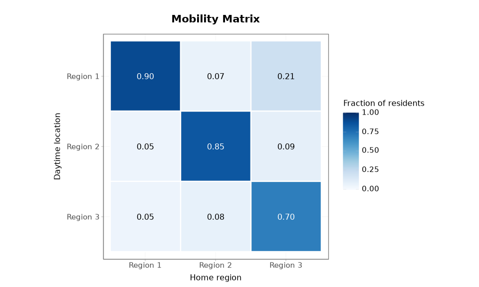
A mobility matrix is a square matrix with one row and one column per region. M[j, k] is the fraction of residents of home region k present at location j. Columns are home regions and each column sums to \(1\). Rows are the same regions, viewed as the locations where residents spend the day; the diagonal is the fraction of residents who stay home. In region 3, 70% of residents stay home on a typical day, 21% spend it in region 1, and 9% in region 2.

• The matrix must represent home regions by column, not rows. A matrix with home regions in its rows, so that each row sums to 1, must be transposed before use, otherwise MobilitySubpopulationInfections rejects it which an error message that says to pass the transpose.
• A matrix stored as a data frame must be converted with .to_numpy(), with rows and columns in that order.
• Regions must be in the same order in the matrix, in subpop_fractions, in a vector-valued I0_rv or log_rt_time_0_rv, and in every observation’s subpop_indices.

You may want to model only some of the areas represented in your raw mobility matrix, or your matrix may include an “everywhere else” bin. To use it in this model, drop any flows to un-modeled locations, then renormalize by columns, so columns once again sum to 1. Roy et al. do this for the twelve local authorities of North East England.

Code

M_full = np.array(
    [
        [0.85, 0.05, 0.10, 0.02],
        [0.05, 0.90, 0.05, 0.03],
        [0.05, 0.03, 0.80, 0.05],
        [0.05, 0.02, 0.05, 0.90],
    ]
)
M_area = M_full[:3, :3]
M_area = M_area / M_area.sum(axis=0, keepdims=True)
print(f"Column sums after renormalizing: {M_area.sum(axis=0)}")

Column sums after renormalizing: [1. 1. 1.]

Building the Latent Process

The latent process takes the matrix as a DeterministicVariable. The matrix is data: it is fixed when the process is constructed and is never estimated.

I0_rv is the number of new incident infections per resident on the first day of the initialization period, the earliest day on the time axis. Infections grow from that value over the initialization period, and every initialization day counts toward susceptible depletion.

Each region starts at its own \(\mathcal{R}(t)\), given as one value per region by log_rt_time_0_rv. Region 2 starts below 1. The random walks have a very small step size, so \(\mathcal{R}(t)\) stays close to its starting value in every region.

Code

gen_int_rv = DeterministicPMF(
    "gen_int", jnp.array([0.16, 0.32, 0.25, 0.14, 0.07, 0.04, 0.02])
)
n_init = 7
I0 = 1e-6
start_rt = jnp.array([1.3, 0.8, 1.2])


def simulate(matrix, susceptible_depletion=True, n_days=120):
    """Simulate one draw of the mobility latent process; return its recorded values."""
    process = MobilitySubpopulationInfections(
        name="mobility",
        gen_int_rv=gen_int_rv,
        n_initialization_points=n_init,
        I0_rv=DeterministicVariable("I0", I0),
        log_rt_time_0_rv=DeterministicVariable("log_rt_time_0", jnp.log(start_rt)),
        baseline_rt_process=RandomWalk(
            innovation_sd_rv=DeterministicVariable("innovation_sd", 0.001),
        ),
        subpop_rt_deviation_process=RandomWalk(
            innovation_sd_rv=DeterministicVariable("innovation_sd", 0.001),
        ),
        mobility_matrix_rv=DeterministicVariable("mobility_matrix", matrix),
        susceptible_depletion=susceptible_depletion,
    )

    def sampler():
        """Sample the latent process and record infections per resident."""
        latent = process.sample(n_days_post_init=n_days, subpop_fractions=p)
        numpyro.deterministic("infections", latent.all_subpops)

    samples = Predictive(sampler, num_samples=1)(random.PRNGKey(0))
    return {
        name.removeprefix("mobility::"): np.asarray(value[0])
        for name, value in samples.items()
    }


def to_long(values, run):
    """Convert a (days, regions) array to a long data frame, after initialization."""
    values = values[n_init:]
    n_days = values.shape[0]
    return pd.DataFrame(
        {
            "day": np.repeat(np.arange(n_days), values.shape[1]),
            "region": np.tile(region_names, n_days),
            "value": values.ravel(),
            "run": run,
        }
    )

Every call to simulate uses the same random key, so the \(\mathcal{R}(t)\) trajectories are the same whatever the matrix.

Mobility Versus No Mobility

With the identity matrix, every resident stays home, and each region follows its own renewal equation. With depletion on, this is the model Roy et al. compare against for regions not linked by mobility.

Code

isolated = simulate(np.eye(3))
linked = simulate(M)

infections_df = pd.concat(
    [
        to_long(isolated["infections"], "Identity matrix"),
        to_long(linked["infections"], "Fig 2b matrix"),
    ]
)

(
    p9.ggplot(infections_df, p9.aes(x="day", y="value", color="run"))
    + p9.geom_line(size=1)
    + p9.facet_wrap("~ region", ncol=3)
    + p9.scale_y_log10()
    + p9.labs(
        x="Days",
        y="New infections per resident",
        title="Infections With and Without Mobility",
        color="",
    )
    + theme_tutorial
    + p9.theme(legend_position="bottom")
)

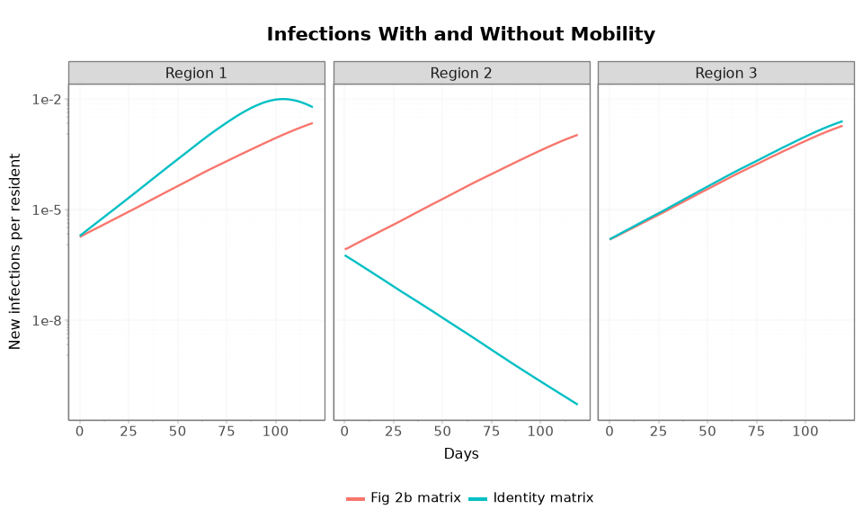
On its own, region 2, with \(\mathcal{R}(t)\) below 1, has a declining epidemic. Linked to the other regions, it has an outbreak: its residents are infected while visiting regions 1 and 3, and infectious visitors from those regions bring infections to region 2. Roy et al. show the same effect in their S2 Fig.

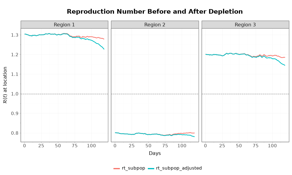
Where \(\mathcal{R}(t)\) Applies

rt_subpop[t, j] is the reproduction number at location j, where transmission happens. It is not the reproduction number of the residents of region j, who are also infected in the regions they visit.

With depletion enabled, rt_subpop_adjusted is the reproduction number at each location after susceptibility adjustment. After the initialization period it is rt_subpop * (share_present @ susceptible_fraction).

Code

rt_df = pd.concat(
    [
        to_long(linked["rt_subpop"], "rt_subpop"),
        to_long(linked["rt_subpop_adjusted"], "rt_subpop_adjusted"),
    ]
)

(
    p9.ggplot(rt_df, p9.aes(x="day", y="value", color="run"))
    + p9.geom_line(size=1)
    + p9.geom_hline(yintercept=1.0, linetype="dashed", color="grey")
    + p9.facet_wrap("~ region", ncol=3)
    + p9.labs(
        x="Days",
        y=r"$\mathcal{R}(t)$ at location",
        title="Reproduction Number Before and After Depletion",
        color="",
    )
    + theme_tutorial
    + p9.theme(legend_position="bottom")
)

Susceptible Depletion

Susceptible depletion is on by default, as in Eq 2.

Code

depleted = simulate(M, susceptible_depletion=True, n_days=250)
not_depleted = simulate(M, susceptible_depletion=False, n_days=250)

susceptible_df = pd.concat(
    [
        to_long(depleted["susceptible_fraction"], "Depletion on"),
        to_long(not_depleted["susceptible_fraction"], "Depletion off"),
    ]
)

(
    p9.ggplot(susceptible_df, p9.aes(x="day", y="value", color="run"))
    + p9.geom_line(size=1)
    + p9.facet_grid("run ~ region", scales="free_y")
    + p9.labs(
        x="Days",
        y="1 - cumulative infections per resident",
        title="Susceptibility With and Without Depletion",
    )
    + p9.guides(color="none")
    + theme_tutorial
    + p9.theme(figure_size=(10, 7))
)

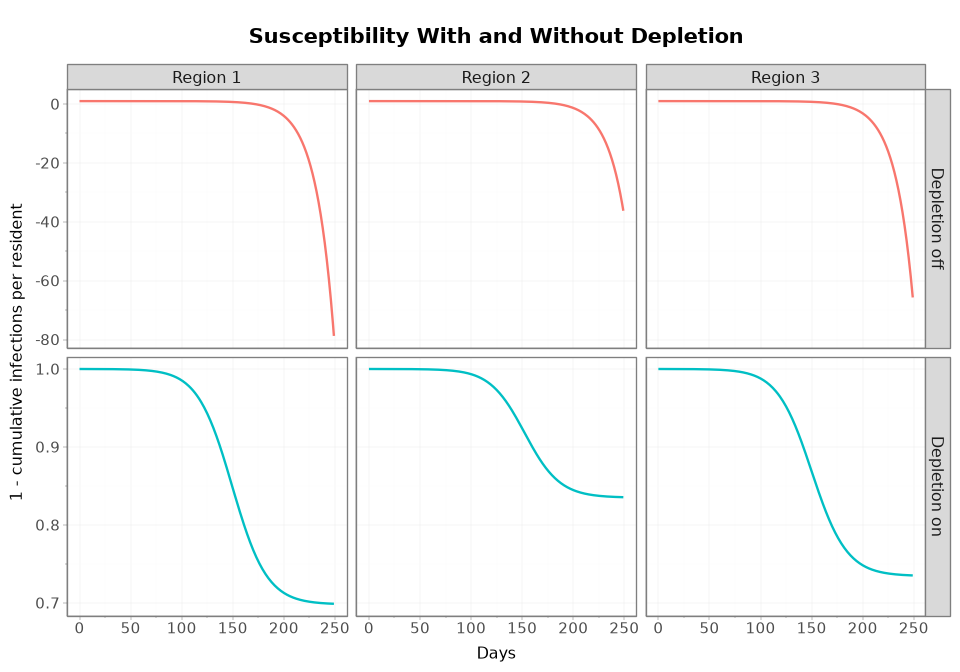
With depletion off, the recorded susceptible fraction becomes negative, indicating that cumulative infections exceed the population. All residents are susceptible at the start of the initialization period, as in Roy et al.

Sources of Infection

Roy et al. (Eqs 3 to 5) split each region’s new infections into three sources:

• local: residents infected at home by infectious residents of the same region;
• incoming: residents infected at home by infectious visitors from other regions;
• outgoing: residents infected while visiting other regions.

PyRenew does not provide a built-in function to compute this split, but it can be computed from recorded values, the matrix, the population fractions, and the generation interval. The generation interval must be fixed, because a sampled one is not recorded.

Code

per_resident = linked["infections"]
rt_subpop = linked["rt_subpop"]
susceptible_fraction = linked["susceptible_fraction"]
reversed_gen_int = np.flip(np.asarray(gen_int_rv()))
n_gen = reversed_gen_int.size
present = M @ p
share_present = M * p[None, :] / np.where(present > 0, present, 1.0)[:, None]

sources = []
for t in range(n_init, per_resident.shape[0]):
    infectiousness = reversed_gen_int @ per_resident[t - n_gen : t]
    at_location = rt_subpop[t] * (share_present @ infectiousness)
    susceptible = susceptible_fraction[t]
    local = (
        susceptible
        * np.diag(M)
        * rt_subpop[t]
        * np.diag(share_present)
        * infectiousness
    )
    incoming = susceptible * np.diag(M) * at_location - local
    new_infections_raw = M.T @ at_location
    outgoing = susceptible * new_infections_raw - local - incoming
    ceiling_scale = 1.0 / np.maximum(new_infections_raw, 1.0)
    sources.append(np.stack([local, incoming, outgoing]) * ceiling_scale)
sources = np.stack(sources)

total = sources.sum(axis=1)
print(
    "Largest absolute difference between the summed sources and the infections: "
    f"{np.max(np.abs(total - per_resident[n_init:])):.1e}"
)

Largest absolute difference between the summed sources and the infections: 4.3e-19

The three sources add up to each day’s new infections, to floating-point precision.

Code

source_names = ["Local", "Incoming", "Outgoing"]
share = np.divide(
    sources,
    total[:, np.newaxis, :],
    out=np.zeros_like(sources),
    where=total[:, np.newaxis, :] > 0,
)
n_days = share.shape[0]
sources_df = pd.DataFrame(
    {
        "day": np.repeat(np.arange(n_days), 9),
        "source": np.tile(np.repeat(source_names, 3), n_days),
        "region": np.tile(region_names, 3 * n_days),
        "share": share.ravel(),
    }
)
sources_df["source"] = pd.Categorical(
    sources_df["source"], categories=source_names, ordered=True
)

(
    p9.ggplot(sources_df, p9.aes(x="day", y="share", fill="source"))
    + p9.geom_area()
    + p9.facet_wrap("~ region", ncol=3)
    + p9.labs(
        x="Days",
        y="Share of new infections",
        title="Sources of New Infections",
        fill="",
    )
    + theme_tutorial
    + p9.theme(legend_position="bottom")
)

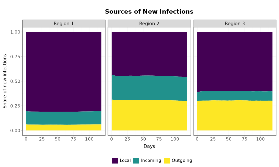
More than half of region 2’s infections come from mobility: its residents are infected while visiting regions with \(\mathcal{R}(t)\) above 1, or at home by visitors from those regions.

Connecting to Observation Processes

MobilitySubpopulationInfections is configured with PyrenewBuilder like SubpopulationInfections, and model.run() takes the same arguments. The matrix is part of the model definition, not run-time data, so fitting and prediction use the same matrix, and no run-time argument can replace it. To model another jurisdiction, build a model with that jurisdiction’s matrix.

Before fitting, run() checks that the matrix has one row and one column per entry of subpop_fractions. Empty locations are allowed and contribute no infections.

For building complete models with observation processes, see:

• Latent Subpopulation Infections
• Observation Processes: Counts
• Building Multi-Signal Models