Latent Subpopulation Infections
Code
import jax.numpy as jnp
import jax.random as random
import numpy as np
import numpyro
from numpyro.infer import Predictive
import pandas as pd
import plotnine as p9
import warnings
from plotnine.exceptions import PlotnineWarning

warnings.filterwarnings("ignore", category=PlotnineWarning)

from _tutorial_theme import theme_tutorial
Code
from pyrenew.latent import (
    SubpopulationInfections,
    AR1,
    DifferencedAR1,
    RandomWalk,
)
from pyrenew.deterministic import DeterministicPMF, DeterministicVariable
Temporal process parameters are RandomVariables. This tutorial uses
DeterministicVariable wrappers to keep those hyperparameters fixed.
Overview
SubpopulationInfections extends the renewal model to a population
composed of \(K\) subpopulations, each with its own latent infection
trajectory.
As in the single-population case, infections evolve according to the renewal equation. For each subpopulation \(k = 1, \dots, K\), we define
where:
- \(I_k(t)\) is the latent infection proportion in subpopulation \(k\) at time \(t\)
- \(\mathcal{R}_k(t)\) is the effective reproduction number for subpopulation \(k\)
- \(w_\tau\) is the generation interval PMF
The generation interval is shared across all subpopulations.
Hierarchical decomposition of \(\mathcal{R}_k(t)\)
The reproduction numbers are modeled through a hierarchical decomposition:
where:
- \(\mathcal{R}_{\text{baseline}}(t)\) is the shared baseline trajectory
- \(\delta_k(t)\) is the deviation for subpopulation \(k\)
This separates:
- shared dynamics via \(\mathcal{R}_{\text{baseline}}(t)\)
- relative differences via \(\delta_k(t)\)
The baseline controls where the epidemic is going, while the deviations control which subpopulations are above or below that trajectory.
Because deviations are additive on the log scale, they act multiplicatively on \(\mathcal{R}_k(t)\): positive \(\delta_k(t)\) increases transmission relative to the baseline, while negative values decrease it.
Aggregation
Each subpopulation produces its own infection trajectory \(I_k(t)\). These are combined into an aggregate infection process using population fractions \(p_k\), where \(p_k\) is the fraction of the total population in subpopulation \(k\), with
The aggregate infection trajectory is then
The aggregate trajectory \(I_{\text{aggregate}}(t)\) is then passed to observation processes, which transform it into expected observations as described in the observation model tutorials.
Relationship to the single-population model
This model generalizes the single-population renewal model:
PopulationInfections: one trajectory \(I(t)\) with one \(\mathcal{R}(t)\)SubpopulationInfections: multiple trajectories \(I_k(t)\) with a shared baseline \(\mathcal{R}_{\text{baseline}}(t)\) and subpopulation deviations \(\delta_k(t)\)
When all \(\delta_k(t) = 0\), the model reduces to the shared (single-population) case.
This tutorial assumes familiarity with the renewal equation, generation
interval, initial conditions (I0, log_rt_time_0), and temporal
processes. See Latent Infections for that
background.
Model Structure
SubpopulationInfections uses the same core inputs as
PopulationInfections, with additional structure for subpopulation
variation.
Core inputs (shared across subpopulations)
gen_int_rv: Generation interval distribution \(w_\tau\)I0_rv: Initial infection level (shared by default across subpopulations, but can be specified per subpopulation)log_rt_time_0_rv: Initial value of \(\log \mathcal{R}_{\text{baseline}}(t)\) at time \(0\)
Temporal processes
Two temporal processes define the evolution of \(\log \mathcal{R}_k(t)\):
-
baseline_rt_processTemporal process for \(\log \mathcal{R}_{\text{baseline}}(t)\). Produces a single trajectory shared across all subpopulations. -
subpop_rt_deviation_processTemporal process for \(\delta_k(t)\). Produces \(K\) trajectories (one per subpopulation), which are centered at each time point to satisfy the sum-to-zero constraint.
Together, these define the full set of reproduction numbers:
Population structure
Population fractions \(p_k\) are provided at sample time, not at model construction. This allows a single model specification to be reused across different jurisdictions or stratifications.
Random variables
As in other PyRenew models, all inputs are specified as
RandomVariables:
DeterministicVariableandDeterministicPMFfor fixed values (used in this tutorial)DistributionalVariablefor parameters with priors (used in inference)
In practice, the temporal processes and initial conditions are typically given prior distributions, allowing the model to infer both shared and subpopulation-specific transmission dynamics.
Code
gen_int_pmf = jnp.array([0.16, 0.32, 0.25, 0.14, 0.07, 0.04, 0.02])
gen_int_rv = DeterministicPMF("gen_int", gen_int_pmf)

subpop_fractions = jnp.array([0.10, 0.14, 0.21, 0.22, 0.07, 0.26])
n_subpops = len(subpop_fractions)

n_days = 28
n_init = len(gen_int_pmf)
n_samples = 200
log_rt_time_0 = 0.2
I0_val = 0.001
rt_cap = 3.0

print(f"Subpopulations: {n_subpops}")
print(f"Population fractions: {np.array(subpop_fractions)}")
print(f"Log Rt at time 0: {np.exp(log_rt_time_0):.2f}")
Subpopulations: 6
Population fractions: [0.1  0.14 0.21 0.22 0.07 0.26]
Log Rt at time 0: 1.22
Code
model = SubpopulationInfections(
    name="SubpopulationInfections",
    gen_int_rv=gen_int_rv,
    I0_rv=DeterministicVariable("I0", I0_val),
    log_rt_time_0_rv=DeterministicVariable("log_rt_time_0", log_rt_time_0),
    baseline_rt_process=DifferencedAR1(
        autoreg_rv=DeterministicVariable("autoreg", 0.5),
        innovation_sd_rv=DeterministicVariable("innovation_sd", 0.01),
    ),
    subpop_rt_deviation_process=AR1(
        autoreg_rv=DeterministicVariable("autoreg", 0.8),
        innovation_sd_rv=DeterministicVariable("innovation_sd", 0.05),
    ),
    n_initialization_points=n_init,
)
The Sum-to-Zero Constraint
Without a constraint, the baseline and deviations are not identifiable:
shifting the baseline up by some amount \(c\) and all deviations down by
\(c\) produces the same subpopulation \(\mathcal{R}_k(t)\) values.
SubpopulationInfections enforces \(\sum_k \delta_k(t) = 0\) at every
time step by centering the raw deviation trajectories. This ensures
\(\mathcal{R}_{\text{baseline}}(t)\) is the unweighted geometric mean of
the subpopulation \(\mathcal{R}_k(t)\) values, so the baseline represents
the typical transmission level across subpopulations.
Note that this is the unweighted mean across subpopulations, not population-weighted by \(p_k\). As a result, \(\mathcal{R}_{\text{baseline}}(t)\) does not in general equal the jurisdiction-level reproduction number implied by the aggregate infection trajectory \(I_{\text{aggregate}}(t)\). When subpopulations differ in size, a small subpopulation with a large \(\mathcal{R}_k(t)\) contributes equally to the baseline but only marginally to the aggregate.
Code
with numpyro.handlers.seed(rng_seed=42):
    with numpyro.handlers.trace() as trace:
        model.sample(
            n_days_post_init=n_days,
            subpop_fractions=subpop_fractions,
        )

deviations = trace["SubpopulationInfections::subpop_deviations"]["value"]
deviation_sums = jnp.sum(deviations, axis=1)
print(f"Deviation shape: {deviations.shape}  (n_total_days, n_subpops)")
print(
    f"Max |sum of deviations across subpops|: {float(jnp.max(jnp.abs(deviation_sums))):.2e}"
)
Deviation shape: (35, 6)  (n_total_days, n_subpops)
Max |sum of deviations across subpops|: 5.22e-08
Choosing the Baseline Temporal Process
The baseline process governs the jurisdiction-level trend in
\(\mathcal{R}(t)\). The same temporal process options apply as in
PopulationInfections (see Temporal Process
Choice): AR(1) for mean
reversion, DifferencedAR1 for persistent trends with stabilizing rate of
change, RandomWalk for unconstrained drift.
We use DifferencedAR1 with small innovation_sd for the baseline
throughout this tutorial. The prior predictive for baseline
\(\mathcal{R}(t)\) behaves much like the corresponding
PopulationInfections example, so we do not repeat that full comparison
here. The focus of this tutorial is the deviation process and how it
changes the spread of subpopulation trajectories around the baseline.
The same high-level decision rules apply here:
| If you believe… | Consider |
|---|---|
| Jurisdiction-wide \(\mathcal{R}(t)\) should stay near a long-run level | AR1 for the baseline |
| Jurisdiction-wide \(\mathcal{R}(t)\) may drift over the modeled horizon | DifferencedAR1 for the baseline |
| Local differences should fade back toward the baseline | AR1 for deviations |
| Local differences can persist or accumulate | RandomWalk for deviations |
Two parameters matter most when tuning these processes:
autoreg: Controls how strongly AR(1)-type processes revert. Values near 1 imply slow reversion; smaller values imply faster pullback.innovation_sd: Controls day-to-day volatility. Larger values produce wider prior spreads and more abrupt movement.
Choosing the Deviation Temporal Process
The deviation process controls how subpopulation \(\mathcal{R}_k(t)\)
values move relative to the baseline \(\mathcal{R}_{\text{baseline}}(t)\),
not the overall trend itself. How \(\delta_k(t)\) behaves at \(t = 0\)
depends on the process. AR1 draws its initial value from the
stationary distribution, so the prior spread of \(\delta_k(0)\) already
matches the stationary standard deviation and stays at that width
throughout. RandomWalk starts at exactly \(\delta_k(0) = 0\) and its
spread grows over time.
The key question: are local differences transient or persistent? This determines whether subpopulations quickly return to the baseline or can diverge and remain different over time.
Code
def sample_hierarchical(baseline_process, deviation_process, label):
    """Draw prior predictive samples from a SubpopulationInfections model."""
    m = SubpopulationInfections(
        name="SubpopulationInfections",
        gen_int_rv=gen_int_rv,
        I0_rv=DeterministicVariable("I0", I0_val),
        log_rt_time_0_rv=DeterministicVariable("log_rt_time_0", log_rt_time_0),
        baseline_rt_process=baseline_process,
        subpop_rt_deviation_process=deviation_process,
        n_initialization_points=n_init,
    )

    def sampler():
        """Wrapper for Predictive."""
        return m.sample(
            n_days_post_init=n_days,
            subpop_fractions=subpop_fractions,
        )

    samples = Predictive(sampler, num_samples=n_samples)(random.PRNGKey(42))
    return {
        "rt_baseline": np.array(samples["SubpopulationInfections::rt_baseline"])[
            :, n_init:, 0
        ],
        "rt_subpop": np.array(samples["SubpopulationInfections::rt_subpop"])[
            :, n_init:, :
        ],
        "deviations": np.array(samples["SubpopulationInfections::subpop_deviations"])[
            :, n_init:, :
        ],
        "infections": np.array(
            samples["SubpopulationInfections::infections_aggregate"]
        )[:, n_init:],
    }


baseline_process = DifferencedAR1(
    autoreg_rv=DeterministicVariable("autoreg", 0.5),
    innovation_sd_rv=DeterministicVariable("innovation_sd", 0.01),
)
AR(1) Deviations
AR(1) deviations have bounded variance. AR1 draws its initial
value from the stationary distribution of the process, so \(\delta_k(0)\)
is already dispersed at the stationary standard deviation
\(\sigma / \sqrt{1 - \phi^2}\) and the envelope stays at that width. With
autoreg = 0.8 and innovation_sd = 0.05, the stationary standard
deviation is approximately \(0.083\) on the log scale.
The autoreg coefficient still matters: if a subpopulation drifts away
from zero by chance, \(\phi\) controls how quickly it is pulled back.
Values near 1 produce slow pullback (local differences linger), values
near 0 produce fast pullback (subpopulations snap back to the baseline).
What this looks like in a prior predictive plot is a constant-width
band rather than a fanning-out cloud.
Code
ar1_dev_samples = sample_hierarchical(
    baseline_process,
    AR1(
        autoreg_rv=DeterministicVariable("autoreg", 0.8),
        innovation_sd_rv=DeterministicVariable("innovation_sd", 0.05),
    ),
    "AR1 deviations",
)
Code
def deviation_df(samples, label):
    """Build a long-format dataframe of deviation trajectories."""
    devs = samples["deviations"]
    data = []
    for i in range(min(50, n_samples)):
        for k in range(n_subpops):
            for d in range(n_days):
                data.append(
                    {
                        "day": d,
                        "deviation": float(devs[i, d, k]),
                        "subpop": f"subpop {k}",
                        "sample": i,
                        "process": label,
                    }
                )
    return pd.DataFrame(data)


def deviation_summary_df(samples):
    """Build a long-format median and 90% interval per (day, subpop) using all samples."""
    devs = samples["deviations"]
    rows = []
    for k in range(n_subpops):
        col = devs[:, :, k]
        for d in range(n_days):
            rows.append(
                {
                    "day": d,
                    "subpop": f"subpop {k}",
                    "median": float(np.median(col[:, d])),
                    "q05": float(np.percentile(col[:, d], 5)),
                    "q95": float(np.percentile(col[:, d], 95)),
                }
            )
    return pd.DataFrame(rows)


ar1_dev_df = deviation_df(ar1_dev_samples, "AR(1) deviations")
ar1_dev_summary = deviation_summary_df(ar1_dev_samples)
Code
(
    p9.ggplot()
    + p9.geom_line(
        ar1_dev_df,
        p9.aes(x="day", y="deviation", group="sample"),
        alpha=0.08,
        size=0.5,
        color="purple",
    )
    + p9.geom_ribbon(
        ar1_dev_summary,
        p9.aes(x="day", ymin="q05", ymax="q95"),
        fill="purple",
        alpha=0.25,
    )
    + p9.geom_line(
        ar1_dev_summary,
        p9.aes(x="day", y="median"),
        color="purple",
        size=0.8,
    )
    + p9.geom_hline(yintercept=0, color="black", linetype="dotted")
    + p9.facet_wrap("~ subpop", ncol=3)
    + p9.coord_cartesian(ylim=(-0.5, 0.5))
    + p9.labs(
        x="Days",
        y="Deviation $\\delta_k(t)$",
        title="AR(1) Deviations (autoreg = 0.8, innovation_sd = 0.05)",
    )
    + theme_tutorial
)
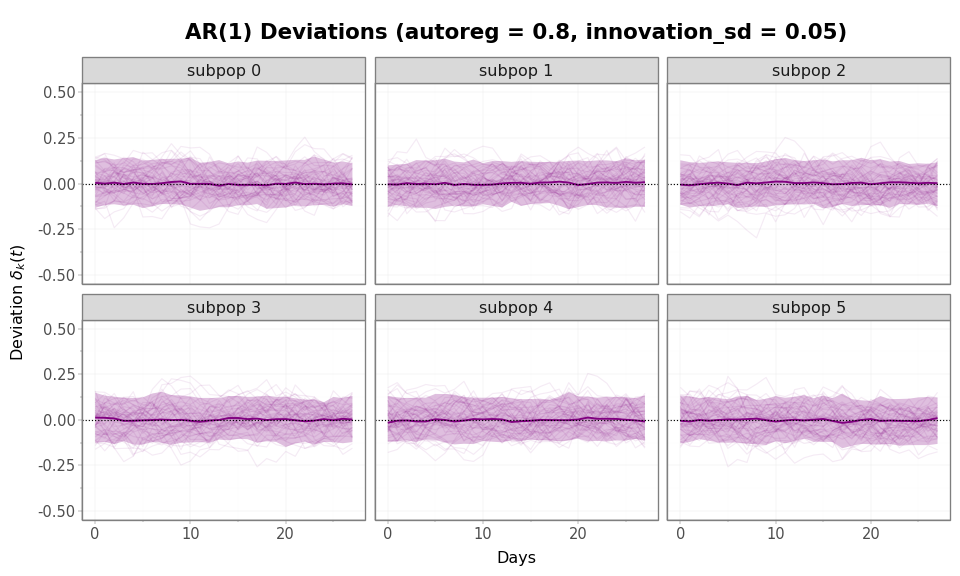
Figure 1: AR(1) deviation trajectories (50 samples, all 6
subpopulations). Because AR1 draws its initial value from the
stationary distribution, the envelope is already at its stationary width
at day 0 and stays bounded there. Compare the y-axis scale to
fig-rw-deviations below.
RandomWalk Deviations
RandomWalk deviations have unbounded variance. The spread of
\(\delta_k(t)\) grows linearly with time as \(\sigma^2 t\), so over a 28-day
horizon with innovation_sd = 0.05 the standard deviation reaches
roughly \(0.265\) on the log scale — about three times the AR(1)
stationary value above. There is no pullback toward zero: subpopulations
that drift away from the baseline stay drifted, and differences that
emerge early persist and can grow. The visual signature is a
fanning-out cloud rather than a constant-width band.
Code
rw_dev_samples = sample_hierarchical(
    baseline_process,
    RandomWalk(
        innovation_sd_rv=DeterministicVariable("innovation_sd", 0.05),
    ),
    "RandomWalk deviations",
)
Code
rw_dev_df = deviation_df(rw_dev_samples, "RandomWalk deviations")
rw_dev_summary = deviation_summary_df(rw_dev_samples)
Code
(
    p9.ggplot()
    + p9.geom_line(
        rw_dev_df,
        p9.aes(x="day", y="deviation", group="sample"),
        alpha=0.08,
        size=0.5,
        color="purple",
    )
    + p9.geom_ribbon(
        rw_dev_summary,
        p9.aes(x="day", ymin="q05", ymax="q95"),
        fill="purple",
        alpha=0.25,
    )
    + p9.geom_line(
        rw_dev_summary,
        p9.aes(x="day", y="median"),
        color="purple",
        size=0.8,
    )
    + p9.geom_hline(yintercept=0, color="black", linetype="dotted")
    + p9.facet_wrap("~ subpop", ncol=3)
    + p9.coord_cartesian(ylim=(-0.5, 0.5))
    + p9.labs(
        x="Days",
        y="Deviation $\\delta_k(t)$",
        title="RandomWalk Deviations (innovation_sd = 0.05)",
    )
    + theme_tutorial
)
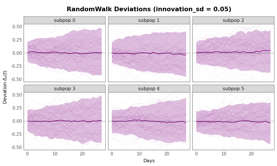
Figure 2: RandomWalk deviation trajectories (50 samples, 6 subpopulations). The envelope fans out continuously over the 28-day horizon and reaches roughly three times the AR(1) stationary width. The y-axis matches fig-ar1-deviations above for direct comparison.
Comparing Deviation Processes
Code
deviation_summary_rows = []
for label, s in [("AR(1)", ar1_dev_samples), ("RandomWalk", rw_dev_samples)]:
    devs = np.abs(s["deviations"][:, -1, :]).flatten()
    deviation_summary_rows.append(
        {
            "Process": label,
            "Median |dev|": f"{np.median(devs):.3f}",
            "90th % |dev|": f"{np.percentile(devs, 90):.3f}",
            "Max |dev|": f"{np.max(devs):.3f}",
        }
    )
pd.DataFrame(deviation_summary_rows)
Table 1: Deviation spread at day 28 (across all subpopulations and samples).
| Process | Median |dev| | 90th % |dev| | Max |dev| | |
|---|---|---|---|---|
| 0 | AR(1) | 0.050 | 0.126 | 0.241 |
| 1 | RandomWalk | 0.184 | 0.432 | 0.823 |
AR(1) deviations stay close to zero because mean reversion continuously pulls them back. RandomWalk deviations accumulate over time. As in the PopulationInfections tutorial, this is prior-modeling guidance rather than a uniquely determined epidemiologic rule. The choice depends on the epidemiological setting:
- AR(1) deviations when subpopulations are expected to track the jurisdiction average. Local outbreaks or lulls are temporary. This is typical for geographically close subpopulations (e.g., counties within a metropolitan area) where mobility mixes transmission.
- RandomWalk deviations when local differences can persist. This may be appropriate for subpopulations with distinct contact patterns, demographics, or intervention histories (e.g., urban vs. rural areas).
Baseline and Deviation Pairs
The baseline and deviation processes interact to determine the full prior over subpopulation \(\mathcal{R}_k(t)\) trajectories. We compare two configurations: DifferencedAR1 baseline with AR(1) deviations, and DifferencedAR1 baseline with RandomWalk deviations.
Code
def subpop_rt_df(samples, label):
    """Build a long-format dataframe of subpopulation Rt trajectories."""
    rt = samples["rt_subpop"]
    rt_base = samples["rt_baseline"]
    data = []
    for i in range(min(50, n_samples)):
        for d in range(n_days):
            data.append(
                {
                    "day": d,
                    "rt": float(rt_base[i, d]),
                    "subpop": "baseline",
                    "sample": i,
                    "config": label,
                }
            )
            for k in range(n_subpops):
                data.append(
                    {
                        "day": d,
                        "rt": float(rt[i, d, k]),
                        "subpop": f"subpop {k}",
                        "sample": i,
                        "config": label,
                    }
                )
    return pd.DataFrame(data)


pairs_df = pd.concat(
    [
        subpop_rt_df(ar1_dev_samples, "DifferencedAR1 + AR(1) deviations"),
        subpop_rt_df(rw_dev_samples, "DifferencedAR1 + RandomWalk deviations"),
    ]
)
Code
baseline_df = pairs_df[pairs_df["subpop"] == "baseline"]
(
    p9.ggplot(baseline_df, p9.aes(x="day", y="rt", group="sample"))
    + p9.geom_line(alpha=0.2, size=0.5, color="steelblue")
    + p9.geom_hline(yintercept=1.0, color="red", linetype="dashed", alpha=0.7)
    + p9.coord_cartesian(ylim=(0, rt_cap))
    + p9.labs(
        x="Days",
        y="Rt (baseline)",
        title=r"Baseline $\mathcal{R}(t)$ (DifferencedAR1, autoreg=0.5, sd=0.01)",
    )
    + theme_tutorial
)
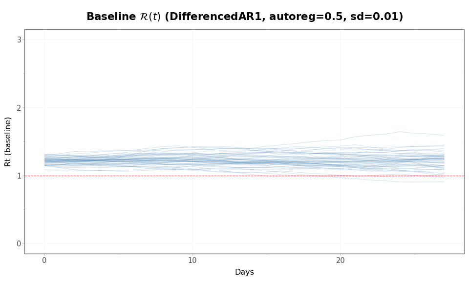
Figure 3: Baseline \(\mathcal{R}(t)\) trajectories are identical for both configurations (same process, same seed). The difference is in how subpopulations spread around this baseline.
Code
def baseline_vs_subpop_summary(samples, subpop_idx, label):
    """Summarize baseline and one subpopulation's Rt across all prior draws."""
    rt_base = samples["rt_baseline"]
    rt_sub = samples["rt_subpop"][:, :, subpop_idx]
    rows = []
    for d in range(n_days):
        rows.append(
            {
                "day": d,
                "series": "baseline",
                "median": float(np.median(rt_base[:, d])),
                "q05": float(np.percentile(rt_base[:, d], 5)),
                "q95": float(np.percentile(rt_base[:, d], 95)),
                "config": label,
            }
        )
        rows.append(
            {
                "day": d,
                "series": "subpop 0",
                "median": float(np.median(rt_sub[:, d])),
                "q05": float(np.percentile(rt_sub[:, d], 5)),
                "q95": float(np.percentile(rt_sub[:, d], 95)),
                "config": label,
            }
        )
    return pd.DataFrame(rows)


config_order = [
    "DifferencedAR1 + AR(1) deviations",
    "DifferencedAR1 + RandomWalk deviations",
]

pairs_summary_df = pd.concat(
    [
        baseline_vs_subpop_summary(ar1_dev_samples, 0, config_order[0]),
        baseline_vs_subpop_summary(rw_dev_samples, 0, config_order[1]),
    ]
)
pairs_summary_df["config"] = pd.Categorical(
    pairs_summary_df["config"], categories=config_order, ordered=True
)

subpop0_df = pairs_df[pairs_df["subpop"] == "subpop 0"].copy()
subpop0_df["config"] = pd.Categorical(
    subpop0_df["config"], categories=config_order, ordered=True
)
baseline_summary = pairs_summary_df[pairs_summary_df["series"] == "baseline"]
subpop_summary = pairs_summary_df[pairs_summary_df["series"] == "subpop 0"]
Code
(
    p9.ggplot()
    + p9.geom_ribbon(
        baseline_summary,
        p9.aes(x="day", ymin="q05", ymax="q95"),
        fill="black",
        alpha=0.15,
    )
    + p9.geom_line(
        subpop0_df,
        p9.aes(x="day", y="rt", group="sample"),
        alpha=0.15,
        size=0.4,
        color="steelblue",
    )
    + p9.geom_ribbon(
        subpop_summary,
        p9.aes(x="day", ymin="q05", ymax="q95"),
        fill="steelblue",
        alpha=0.3,
    )
    + p9.geom_line(
        baseline_summary,
        p9.aes(x="day", y="median"),
        color="black",
        size=1.0,
    )
    + p9.geom_line(
        subpop_summary,
        p9.aes(x="day", y="median"),
        color="steelblue",
        size=1.0,
    )
    + p9.geom_hline(yintercept=1.0, color="red", linetype="dashed", alpha=0.7)
    + p9.facet_wrap("~ config", ncol=2)
    + p9.scale_y_log10(limits=(0.5, rt_cap))
    + p9.labs(
        x="Days",
        y=r"$\mathcal{R}(t)$ (log scale)",
        title=r"Subpopulation 0 $\mathcal{R}(t)$ vs Baseline Under Two Deviation Process Choices",
    )
    + theme_tutorial
)
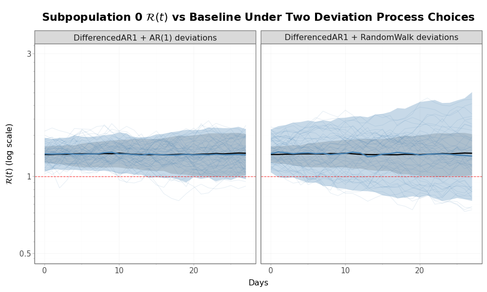
Figure 4: Prior predictive bands for subpopulation 0’s \(\mathcal{R}(t)\) (blue) overlaid on the shared baseline \(\mathcal{R}_{\text{baseline}}(t)\) (black), under two deviation process choices. Each panel shows 50 subpopulation 0 trajectories (light blue lines), the 5–95% prior interval for subpopulation 0 (blue ribbon) and for the baseline (grey ribbon), and their medians (solid lines). The y-axis is log-scaled so that additive log-deviations appear as constant multiplicative widths. With AR(1) deviations (left), the subpopulation band has nearly the same width as the baseline band at every day, because the deviation variance is stationary. With RandomWalk deviations (right), the subpopulation band widens relative to the baseline band as the horizon grows, because deviation variance accumulates.
Code
single_draw_data = []
for label, s in [
    ("DifferencedAR1 +\nAR(1) deviations", ar1_dev_samples),
    ("DifferencedAR1 +\nRandomWalk deviations", rw_dev_samples),
]:
    rt_base = s["rt_baseline"][0, :]
    rt_sub = s["rt_subpop"][0, :, :]
    for d in range(n_days):
        single_draw_data.append(
            {
                "day": d,
                "rt": float(rt_base[d]),
                "subpop": "baseline",
                "config": label,
            }
        )
        for k in range(n_subpops):
            single_draw_data.append(
                {
                    "day": d,
                    "rt": float(rt_sub[d, k]),
                    "subpop": f"subpop {k}",
                    "config": label,
                }
            )

single_draw_df = pd.DataFrame(single_draw_data)
single_draw_df["config"] = pd.Categorical(
    single_draw_df["config"],
    categories=[
        "DifferencedAR1 +\nAR(1) deviations",
        "DifferencedAR1 +\nRandomWalk deviations",
    ],
    ordered=True,
)
(
    p9.ggplot(single_draw_df, p9.aes(x="day", y="rt", color="subpop"))
    + p9.geom_line(
        single_draw_df[single_draw_df["subpop"] != "baseline"],
        alpha=0.6,
        size=0.5,
    )
    + p9.geom_line(
        single_draw_df[single_draw_df["subpop"] == "baseline"],
        size=1.2,
        color="black",
    )
    + p9.facet_wrap("~ config", ncol=2)
    + p9.coord_cartesian(ylim=(0, rt_cap))
    + p9.labs(
        x="Days",
        y="Rt",
        title=r"Single Prior Draw: Baseline (black) and Subpopulation $\mathcal{R}(t)$",
        color="",
    )
    + theme_tutorial
    + p9.theme(legend_position="bottom")
)
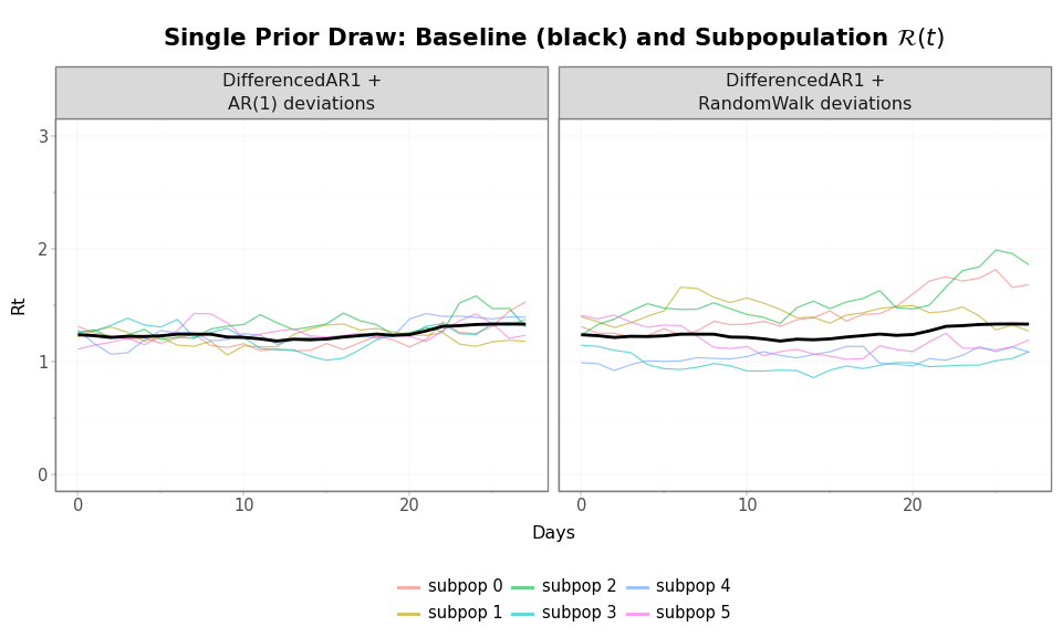
Figure 5: All 6 subpopulation \(\mathcal{R}(t)\) trajectories from a single prior draw, under both configurations. AR(1) deviations (left) keep subpopulations tightly bundled; RandomWalk deviations (right) allow them to spread apart.
Connecting to Observation Processes
The latent infection trajectory is not observed directly. Each
observation process selects a subset of subpopulations (via
subpop_indices) and applies its own ascertainment rate and delay
distribution.
The PyrenewBuilder handles the wiring:
configure_latent()sets the hierarchical infection process (called once)add_observation()adds an observation process, specifying which subpopulations it observes (called once per data stream)build()computesn_initialization_pointsfrom all delay distributions and produces a model ready for inference
To learn how to build complete models with observation processes, see: