Day-of-week effects for count data

Code

import jax.numpy as jnp
import numpy as np
import numpyro
import pandas as pd

from pyrenew.observation import Counts, NegativeBinomialNoise, PoissonNoise
from pyrenew.deterministic import DeterministicVariable, DeterministicPMF
from pyrenew import datasets

import plotnine as p9
from plotnine.exceptions import PlotnineWarning
import warnings

warnings.filterwarnings("ignore", category=PlotnineWarning)

from _tutorial_theme import theme_tutorial

Many health surveillance signals exhibit strong day-of-week patterns. Emergency department visits and hospital admissions tend to be higher on weekdays and lower on weekends, driven by staffing, patient behavior, and reporting practices. Ignoring this weekly periodicity forces the noise model to absorb systematic variation, inflating dispersion estimates and obscuring the underlying epidemic trend.

PyRenew models day-of-week effects as a multiplicative adjustment applied to predicted counts after the delay convolution and ascertainment scaling:

\[\lambda(t) = d_{w(t)} \cdot \alpha \sum_{s} I(t-s)\,\pi(s)\]

where \(d_{w(t)}\) is the day-of-week multiplier for the weekday of timepoint \(t\), \(\alpha\) is the ascertainment rate, and \(\pi(s)\) is the delay PMF. The effect vector \(\mathbf{d} = (d_0, d_1, \ldots, d_6)\) has one entry per day (0=Monday through 6=Sunday, ISO convention). An effect of 1.0 means no adjustment for that day. When the effects sum to 7.0, the average daily multiplier is 1.0, preserving weekly totals and keeping the ascertainment rate directly interpretable as the fraction of infections observed.

Defining a day-of-week effect

A typical pattern for ED visits might show weekday effects above 1.0 and weekend effects below 1.0:

Code

dow_values = jnp.array([1.20, 1.15, 1.10, 1.05, 1.00, 0.75, 0.75])
day_names = ["Mon", "Tue", "Wed", "Thu", "Fri", "Sat", "Sun"]

print(f"Day-of-week effects: {np.round(np.array(dow_values), 2)}")
print(f"Sum: {float(jnp.sum(dow_values)):.2f}")

Day-of-week effects: [1.2  1.15 1.1  1.05 1.   0.75 0.75]
Sum: 7.00

Code

dow_df = pd.DataFrame({"day": day_names, "effect": np.array(dow_values)})
dow_df["day"] = pd.Categorical(
    dow_df["day"], categories=day_names, ordered=True
)

(
    p9.ggplot(dow_df, p9.aes(x="day", y="effect"))
    + p9.geom_col(fill="steelblue", alpha=0.7, color="black")
    + p9.geom_hline(yintercept=1.0, linetype="dashed", color="grey")
    + p9.labs(
        x="Day of Week",
        y="Multiplicative Effect",
        title="Day-of-Week Effect Vector",
    )
    + theme_tutorial
)

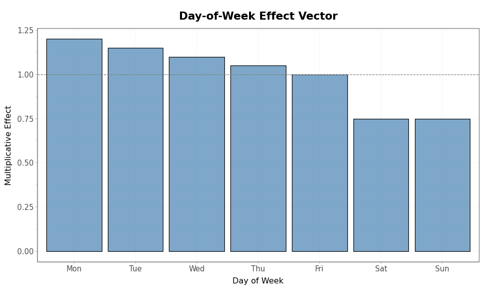
Values above the dashed line (1.0) increase predicted counts for that day; values below decrease them. Monday at 1.20 means 20% more counts than an average day; Saturday and Sunday at 0.75 mean 25% fewer.

Observation process with and without day-of-week effects

We construct two Counts observation processes using the same delay distribution and ascertainment rate. The only difference is whether day_of_week_rv is provided.

Code

hosp_delay_pmf = jnp.array(
    datasets.load_infection_admission_interval()["probability_mass"].to_numpy()
)
delay_rv = DeterministicPMF("inf_to_hosp_delay", hosp_delay_pmf)
ihr_rv = DeterministicVariable("ihr", 0.01)
concentration_rv = DeterministicVariable("concentration", 20.0)

process_no_dow = Counts(
    name="hosp_no_dow",
    ascertainment_rate_rv=ihr_rv,
    delay_distribution_rv=delay_rv,
    noise=NegativeBinomialNoise(concentration_rv),
)

process_with_dow = Counts(
    name="hosp_dow",
    ascertainment_rate_rv=ihr_rv,
    delay_distribution_rv=delay_rv,
    noise=NegativeBinomialNoise(concentration_rv),
    day_of_week_rv=DeterministicVariable("dow_effect", dow_values),
)

We simulate a growing epidemic and generate predicted counts from both processes. The first_day_dow parameter tells PyRenew which day of the week corresponds to element 0 of the time axis. Here we set first_day_dow=0 (Monday).

Code

day_one = process_no_dow.lookback_days()
n_total = 130
infections = 5000.0 * jnp.exp(0.03 * jnp.arange(n_total))

with numpyro.handlers.seed(rng_seed=0):
    result_no_dow = process_no_dow.sample(infections=infections, obs=None)
with numpyro.handlers.seed(rng_seed=0):
    result_with_dow = process_with_dow.sample(
        infections=infections, obs=None, first_day_dow=0
    )

Code

n_plot_days = n_total - day_one
pred_rows = []
for i in range(n_plot_days):
    day_idx = day_one + i
    pred_rows.append(
        {
            "day": i,
            "admissions": float(result_no_dow.predicted[day_idx]),
            "type": "No day-of-week effect",
        }
    )
    pred_rows.append(
        {
            "day": i,
            "admissions": float(result_with_dow.predicted[day_idx]),
            "type": "With day-of-week effect",
        }
    )
pred_df = pd.DataFrame(pred_rows)
pred_df["type"] = pd.Categorical(
    pred_df["type"],
    categories=["No day-of-week effect", "With day-of-week effect"],
    ordered=True,
)

(
    p9.ggplot(
        pred_df, p9.aes(x="day", y="admissions", color="type", linetype="type")
    )
    + p9.geom_line(size=1)
    + p9.scale_color_manual(values=["steelblue", "#e41a1c"])
    + p9.scale_linetype_manual(values=["solid", "dashed"])
    + p9.labs(
        x="Day",
        y="Predicted Admissions",
        title="Predicted Admissions:\nWith vs. Without Day-of-Week Effect",
        color="",
        linetype="",
    )
    + theme_tutorial
)

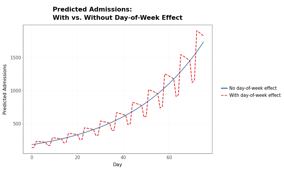
Without the day-of-week effect the predicted curve is smooth. With it, the curve oscillates with a 7-day period — dipping on weekends and rising on weekdays — while following the same overall trend.

Effect of the offset

The first_day_dow parameter aligns the weekly pattern to the calendar. Changing it shifts which days receive which multiplier. Here we compare starting on Monday vs. Wednesday:

Code

with numpyro.handlers.seed(rng_seed=0):
    result_monday = process_with_dow.sample(
        infections=infections, obs=None, first_day_dow=0
    )
with numpyro.handlers.seed(rng_seed=0):
    result_wednesday = process_with_dow.sample(
        infections=infections, obs=None, first_day_dow=2
    )

Code

offset_rows = []
for i in range(21):
    day_idx = day_one + i
    offset_rows.append(
        {
            "day": i,
            "admissions": float(result_monday.predicted[day_idx]),
            "offset": "first_day_dow=0 (Monday)",
        }
    )
    offset_rows.append(
        {
            "day": i,
            "admissions": float(result_wednesday.predicted[day_idx]),
            "offset": "first_day_dow=2 (Wednesday)",
        }
    )
offset_df = pd.DataFrame(offset_rows)
offset_df["offset"] = pd.Categorical(
    offset_df["offset"],
    categories=[
        "first_day_dow=0 (Monday)",
        "first_day_dow=2 (Wednesday)",
    ],
    ordered=True,
)

(
    p9.ggplot(
        offset_df,
        p9.aes(x="day", y="admissions", color="offset"),
    )
    + p9.geom_line(size=1)
    + p9.geom_point(size=2)
    + p9.scale_color_manual(values=["steelblue", "#e41a1c"])
    + p9.labs(
        x="Day",
        y="Predicted Admissions",
        title="Effect of first_day_dow on Weekly Pattern Alignment",
        color="",
    )
    + theme_tutorial
)

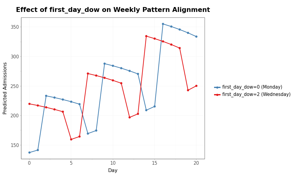
The two curves have the same shape but are phase-shifted: their weekend dips fall on different days. Getting first_day_dow right matters — a misaligned offset would attribute Monday’s high to Sunday or vice versa.

When using MultiSignalModel, the shared time axis starts n_init days before the first observation. The convenience method model.compute_first_day_dow(obs_start_dow) converts the known day of the week of the first observation to the correct offset for element 0 of the time axis.

Sampled observations

Day-of-week effects shape the noise draws, not just the predicted means. The noise model samples from a distribution centered on the adjusted predictions, so sampled observations inherit the weekly pattern.

Code

n_samples = 30
noisy_results = []
for seed in range(n_samples):
    with numpyro.handlers.seed(rng_seed=seed):
        result_no = process_no_dow.sample(infections=infections, obs=None)
    with numpyro.handlers.seed(rng_seed=seed):
        result_yes = process_with_dow.sample(
            infections=infections, obs=None, first_day_dow=0
        )
    for i in range(n_plot_days):
        day_idx = day_one + i
        noisy_results.append(
            {
                "day": i,
                "admissions": float(result_no.observed[day_idx]),
                "type": "No day-of-week effect",
                "sample": seed,
            }
        )
        noisy_results.append(
            {
                "day": i,
                "admissions": float(result_yes.observed[day_idx]),
                "type": "With day-of-week effect",
                "sample": seed,
            }
        )

Code

noisy_df = pd.DataFrame(noisy_results)
mean_df = noisy_df.groupby(["day", "type"])["admissions"].mean().reset_index()

(
    p9.ggplot(noisy_df, p9.aes(x="day", y="admissions"))
    + p9.geom_line(
        p9.aes(group="sample"), alpha=0.15, size=0.4, color="steelblue"
    )
    + p9.geom_line(
        data=mean_df,
        mapping=p9.aes(x="day", y="admissions"),
        color="#e41a1c",
        size=1.2,
    )
    + p9.facet_wrap("~ type", ncol=1)
    + p9.labs(
        x="Day",
        y="Hospital Admissions",
        title="Sampled Observations:\nWith vs. Without Day-of-Week Effect",
    )
    + theme_tutorial
)

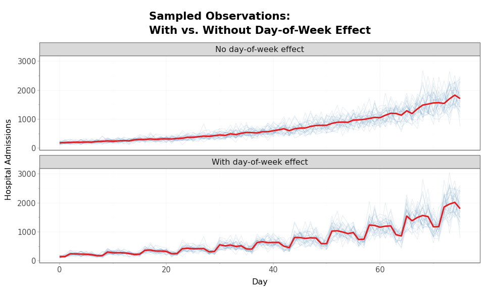
The top panel shows smooth variation around the trend. The bottom panel shows systematic weekly oscillation in both the mean (red) and individual samples (blue) — the weekend dips are visible even through the noise.

Composing with right-truncation

Day-of-week effects and right-truncation are independent adjustments that compose naturally. Day-of-week is applied first (adjusting the expected counts for reporting patterns), then right-truncation scales down recent counts for incomplete reporting:

\[\lambda(t) = F(k_t) \cdot d_{w(t)} \cdot \alpha \sum_s I(t-s)\,\pi(s)\]

Code

reporting_delay_pmf = jnp.array([0.4, 0.3, 0.15, 0.08, 0.04, 0.02, 0.01])

process_both = Counts(
    name="hosp_both",
    ascertainment_rate_rv=ihr_rv,
    delay_distribution_rv=delay_rv,
    noise=NegativeBinomialNoise(concentration_rv),
    day_of_week_rv=DeterministicVariable("dow_effect", dow_values),
    right_truncation_rv=DeterministicPMF(
        "reporting_delay", reporting_delay_pmf
    ),
)

with numpyro.handlers.seed(rng_seed=0):
    result_both = process_both.sample(
        infections=infections,
        obs=None,
        first_day_dow=0,
        right_truncation_offset=0,
    )

Code

compose_rows = []
for i in range(n_plot_days):
    day_idx = day_one + i
    compose_rows.append(
        {
            "day": i,
            "admissions": float(result_with_dow.predicted[day_idx]),
            "type": "Day-of-week only",
        }
    )
    compose_rows.append(
        {
            "day": i,
            "admissions": float(result_both.predicted[day_idx]),
            "type": "Day-of-week + right-truncation",
        }
    )
compose_df = pd.DataFrame(compose_rows)
compose_df["type"] = pd.Categorical(
    compose_df["type"],
    categories=["Day-of-week only", "Day-of-week + right-truncation"],
    ordered=True,
)

(
    p9.ggplot(
        compose_df,
        p9.aes(x="day", y="admissions", color="type", linetype="type"),
    )
    + p9.geom_line(size=1)
    + p9.scale_color_manual(values=["steelblue", "#e41a1c"])
    + p9.scale_linetype_manual(values=["solid", "dashed"])
    + p9.labs(
        x="Day",
        y="Predicted Admissions",
        title="Day-of-Week Effect Composed with Right-Truncation",
        color="",
        linetype="",
    )
    + theme_tutorial
)

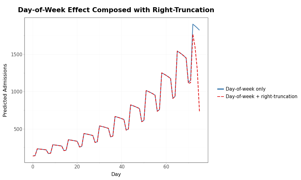
The two curves agree in the early period. Near the right edge, right-truncation pulls the curve downward on top of the weekly oscillation. Each adjustment operates on its own concern — weekly reporting patterns vs. incomplete recent data — and they combine multiplicatively without interfering.

Summary

Day-of-week adjustment is enabled by passing a day_of_week_rv at construction time and a first_day_dow at sample time.

Parameter	Where	Purpose
day_of_week_rv	Constructor	7-element multiplicative effect vector (0=Mon, 6=Sun)
first_day_dow	sample()	Day of the week for element 0 of the time axis

When either is None, the adjustment is disabled and the process behaves identically to one without day-of-week effects.

The effect vector can be supplied as a fixed DeterministicVariable from empirical data, or as a stochastic RandomVariable (e.g., a scaled Dirichlet prior) to infer the weekly pattern from data. Effects summing to 7.0 preserve weekly totals and keep the ascertainment rate interpretable; other sums rescale overall predicted counts.