Right-truncation adjustment for count data

Code

import jax.numpy as jnp
import numpy as np
import numpyro
import pandas as pd

from pyrenew.observation import Counts, NegativeBinomialNoise
from pyrenew.deterministic import DeterministicVariable, DeterministicPMF
from pyrenew.convolve import compute_prop_already_reported
from pyrenew import datasets

import plotnine as p9
from plotnine.exceptions import PlotnineWarning
import warnings

warnings.filterwarnings("ignore", category=PlotnineWarning)

from _tutorial_theme import theme_tutorial

Right-truncation occurs when recent observations are incomplete because not all events have been reported yet. In hospital surveillance, an admission that occurred \(d\) days ago may not yet appear in the data if the reporting delay exceeds \(d\) days. Ignoring this produces a spurious decline in recent counts.

PyRenew’s observation equation defines the expected observation count as:

\[\mu(t) = \alpha \sum_{s} I(t-s) \, \pi(s)\]

where \(\alpha\) is the ascertainment rate and \(\pi(s)\) is the infection-to-observation delay distribution.

Right-truncation introduces a second delay: the reporting delay, which is the time from the clinical event to its appearance in the data system. PyRenew models this as a multiplicative adjustment applied after the delay convolution. The predicted observation rate becomes:

\[\lambda(t) = F(k_t) \cdot \mu(t)\]

where \(F\) is the CDF of the reporting delay and \(k_t\) is the number of days between timepoint \(t\) and the data pull date (the date on which the dataset was extracted from the surveillance system). Concretely, let \(T\) denote the last observation day and let \(\text{offset} = \text{data pull date} - T\) be the number of additional days between day \(T\) and the data pull (the right_truncation_offset parameter). Then:

\[k_t = (T - t) + \text{offset} = (T - t) + (\text{data pull date} - T) = \text{data pull date} - t\]

Because \(k_t\) depends only on the data pull date and the timepoint \(t\), its behavior is straightforward: timepoints far in the past (small \(t\)) have large \(k_t\), so \(F(k_t) \approx 1\) and counts are fully reported. Recent timepoints (large \(t\), close to the data pull date) have small \(k_t\) and \(F(k_t) < 1\), reducing the predicted counts to reflect incomplete reporting.

Reporting delay and proportion already reported

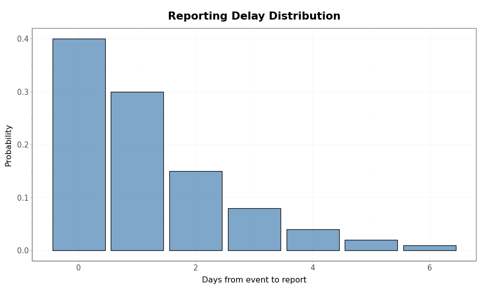
The reporting delay PMF specifies how quickly events are reported. Given this PMF and the number of days between each timepoint and the data pull date, compute_prop_already_reported returns the proportion of events already reported at each timepoint.

Code

reporting_delay_pmf = jnp.array([0.4, 0.3, 0.15, 0.08, 0.04, 0.02, 0.01])

days_pmf = np.arange(len(reporting_delay_pmf))
cdf = np.cumsum(np.array(reporting_delay_pmf))
mean_delay = float(np.sum(days_pmf * reporting_delay_pmf))
print(f"Reporting delay PMF support: 0 to {len(reporting_delay_pmf) - 1} days")
print(f"Mean reporting delay: {mean_delay:.1f} days")
print(f"CDF: {np.round(cdf, 2)}")

Reporting delay PMF support: 0 to 6 days
Mean reporting delay: 1.2 days
CDF: [0.4  0.7  0.85 0.93 0.97 0.99 1.  ]

Code

delay_df = pd.DataFrame(
    {"day": days_pmf, "probability": np.array(reporting_delay_pmf)}
)

(
    p9.ggplot(delay_df, p9.aes(x="day", y="probability"))
    + p9.geom_col(fill="steelblue", alpha=0.7, color="black")
    + p9.labs(
        x="Days from event to report",
        y="Probability",
        title="Reporting Delay Distribution",
    )
    + theme_tutorial
)

The right_truncation_offset parameter specifies how many additional days of reporting have elapsed beyond the last observation. An offset of 0 means the data was pulled on the same day as the last observation — only delay-0 reports have arrived for that day. An offset of 3 means three additional days have passed, allowing more reports to trickle in.

Code

n_example = 20
offsets = [0, 2, 4]

prop_results = []
for offset in offsets:
    prop = compute_prop_already_reported(
        reporting_delay_pmf, n_example, offset
    )
    for i in range(n_example):
        prop_results.append(
            {
                "day": i,
                "proportion": float(prop[i]),
                "offset": f"offset = {offset}",
            }
        )

Code

prop_df = pd.DataFrame(prop_results)
prop_df["offset"] = pd.Categorical(
    prop_df["offset"],
    categories=[f"offset = {o}" for o in offsets],
    ordered=True,
)

(
    p9.ggplot(prop_df, p9.aes(x="day", y="proportion", color="offset"))
    + p9.geom_line(size=1)
    + p9.geom_point(size=2)
    + p9.scale_color_manual(values=["#e41a1c", "#377eb8", "#4daf4a"])
    + p9.ylim(0, 1.05)
    + p9.labs(
        x="Day",
        y="Proportion Already Reported",
        title="Right-Truncation Adjustment by Offset",
        color="",
    )
    + theme_tutorial
)

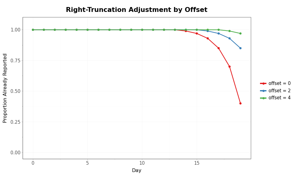
With offset 0, the most recent days are substantially underreported. Larger offsets mean more time has elapsed for reports to arrive, shifting the truncation window forward.

Observation process with and without right-truncation

We construct two Counts observation processes: one without right-truncation (the default) and one with a right_truncation_rv that supplies the reporting delay PMF.

Code

hosp_delay_pmf = jnp.array(
    datasets.load_infection_admission_interval()["probability_mass"].to_numpy()
)
delay_rv = DeterministicPMF("inf_to_hosp_delay", hosp_delay_pmf)
ihr_rv = DeterministicVariable("ihr", 0.01)
concentration_rv = DeterministicVariable("concentration", 10.0)

process_no_trunc = Counts(
    name="hosp_no_trunc",
    ascertainment_rate_rv=ihr_rv,
    delay_distribution_rv=delay_rv,
    noise=NegativeBinomialNoise(concentration_rv),
)

process_with_trunc = Counts(
    name="hosp_trunc",
    ascertainment_rate_rv=ihr_rv,
    delay_distribution_rv=delay_rv,
    noise=NegativeBinomialNoise(concentration_rv),
    right_truncation_rv=DeterministicPMF(
        "reporting_delay", reporting_delay_pmf
    ),
)

We simulate an epidemic that is still growing at the end of the observation window.

Code

day_one = process_no_trunc.lookback_days()
n_total = 80
n_plot_days = n_total - day_one
infections = 5000.0 * jnp.exp(0.04 * jnp.arange(n_total))

with numpyro.handlers.seed(rng_seed=0):
    result_no_trunc = process_no_trunc.sample(infections=infections, obs=None)
with numpyro.handlers.seed(rng_seed=0):
    result_trunc = process_with_trunc.sample(
        infections=infections, obs=None, right_truncation_offset=0
    )

The plot below overlays predicted admissions with and without right-truncation so the early agreement and late divergence are easy to see.

Code

pred_rows = []
for i in range(n_plot_days):
    pred_rows.append(
        {
            "day": i,
            "admissions": float(result_no_trunc.predicted[day_one + i]),
            "type": "Complete reporting",
        }
    )
    pred_rows.append(
        {
            "day": i,
            "admissions": float(result_trunc.predicted[day_one + i]),
            "type": "Right-truncated (offset=0)",
        }
    )
pred_df = pd.DataFrame(pred_rows)
pred_df["type"] = pd.Categorical(
    pred_df["type"],
    categories=["Complete reporting", "Right-truncated (offset=0)"],
    ordered=True,
)

(
    p9.ggplot(
        pred_df, p9.aes(x="day", y="admissions", color="type", linetype="type")
    )
    + p9.geom_line(size=1)
    + p9.scale_color_manual(values=["steelblue", "#e41a1c"])
    + p9.scale_linetype_manual(values=["solid", "dashed"])
    + p9.labs(
        x="Day",
        y="Predicted Admissions",
        title="Predicted Hospital Admissions",
        color="",
        linetype="",
    )
    + theme_tutorial
)

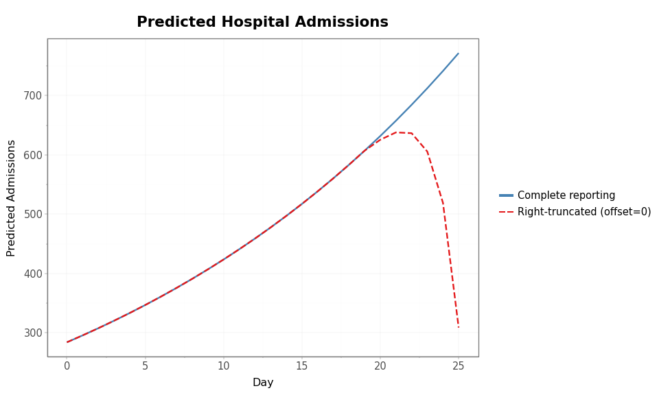
The two curves agree perfectly in the early period when all reports have arrived. Near the right edge the truncated curve turns downward — recent counts are depressed because reports have not yet arrived. Without the right-truncation adjustment, a model fit to the dashed curve would infer that the epidemic is slowing down — a dangerous misinterpretation during an active outbreak.

Sampled observations

Right-truncation also affects the sampled (noisy) observations, not just the predicted means. The noise model draws from a distribution centered on the adjusted predictions.

Code

n_samples = 30
noisy_results = []
for seed in range(n_samples):
    with numpyro.handlers.seed(rng_seed=seed):
        result_no = process_no_trunc.sample(infections=infections, obs=None)
    with numpyro.handlers.seed(rng_seed=seed):
        result_tr = process_with_trunc.sample(
            infections=infections, obs=None, right_truncation_offset=0
        )
    for i in range(n_plot_days):
        noisy_results.append(
            {
                "day": i,
                "admissions": float(result_no.observed[day_one + i]),
                "type": "Complete reporting",
                "sample": seed,
            }
        )
        noisy_results.append(
            {
                "day": i,
                "admissions": float(result_tr.observed[day_one + i]),
                "type": "Right-truncated (offset=0)",
                "sample": seed,
            }
        )

Code

noisy_df = pd.DataFrame(noisy_results)
mean_df = noisy_df.groupby(["day", "type"])["admissions"].mean().reset_index()

(
    p9.ggplot(noisy_df, p9.aes(x="day", y="admissions"))
    + p9.geom_line(
        p9.aes(group="sample"), alpha=0.2, size=0.4, color="steelblue"
    )
    + p9.geom_line(
        data=mean_df,
        mapping=p9.aes(x="day", y="admissions"),
        color="#e41a1c",
        size=1.2,
    )
    + p9.facet_wrap("~ type", ncol=1)
    + p9.labs(
        x="Day",
        y="Hospital Admissions",
        title="Sampled Observations:\nWith vs. Without Right-Truncation",
    )
    + theme_tutorial
)

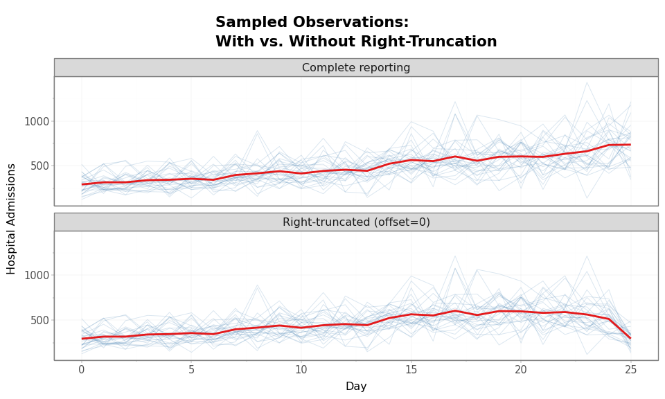
The red line is the mean across samples. In the top panel (complete reporting), the mean tracks the growing epidemic. In the bottom panel (right-truncated), the mean turns downward at the right edge — a spurious decline caused entirely by incomplete reporting.

Summary

Right-truncation adjustment is enabled by passing a right_truncation_rv (reporting delay PMF) at construction time and a right_truncation_offset at sample time.

Parameter	Where	Purpose
right_truncation_rv	Constructor	Reporting delay PMF
right_truncation_offset	sample()	Days between last observation and data pull

When either is None, the adjustment is disabled and the process behaves identically to one without right-truncation. This makes it straightforward to compare models with and without the adjustment, or to supply the reporting delay as either a fixed PMF or an inferred distribution.

In practice, right-truncation adjustment should be enabled when fitting to observed data, so the model correctly attributes low recent counts to incomplete reporting rather than a true decline. However, it should be disabled when forecasting: future timepoints have not yet occurred, so there is no reporting delay to account for — applying the adjustment would nonsensically shrink forecasted counts toward zero. A typical workflow is to fit with right_truncation_offset set to the actual offset, then generate forecasts with right_truncation_offset=None.