Joint ascertainment
Code
import jax.nn as jnn
import jax.numpy as jnp
import jax.random as random
import numpy as np
import numpyro
import numpyro.distributions as dist
import pandas as pd
import plotnine as p9
import warnings
from plotnine.exceptions import PlotnineWarning
from _tutorial_theme import theme_tutorial

from pyrenew.ascertainment import JointAscertainment
from pyrenew.deterministic import DeterministicPMF
from pyrenew.model import PyrenewBuilder
from pyrenew.observation import NegativeBinomialNoise, PopulationCounts
from pyrenew.randomvariable import DistributionalVariable
from pyrenew.time import MMWR_WEEK

warnings.filterwarnings("ignore", category=PlotnineWarning)
Ascertainment is the probability that a latent infection appears in an observed signal, e.g., a hospitalization or visit to the emergency department. For hospital admissions this probability is often called an infection-hospitalization rate (IHR). For emergency department visits it might be called an infection-ED-visit rate (IEDR).
PyRenew count observations accept an ascertainment_rate_rv. For simple
models this can be any ordinary RandomVariable.
For multi-signal models, PyRenew also provides model-level ascertainment components that let multiple observation processes share related ascertainment structure. These components are intended for count signals whose observation probabilities are logically related because they are different event streams generated from the same latent infections. Hospital admissions and ED visits are a natural example: they have different observation probabilities, but both depend on clinical care-seeking and reporting.
Independent scalar ascertainment
Before considering multi-signal models with related ascertainment structure, we show how to specify a multi-signal model where the signals are modeled independently. In this model, each observation process has its own scalar ascertainment prior.
Code
hosp_delay_pmf = jnp.array([0.05, 0.10, 0.15, 0.15, 0.20, 0.15, 0.15, 0.05])
hosp_delay_rv = DeterministicPMF("inf_to_hosp_delay", hosp_delay_pmf)

ed_delay_pmf = jnp.array([0.05, 0.15, 0.30, 0.30, 0.15, 0.05])
ed_delay_rv = DeterministicPMF("inf_to_ed_delay", ed_delay_pmf)

hospital_obs_independent = PopulationCounts(
    name="hospital",
    ascertainment_rate_rv=DistributionalVariable("ihr", dist.Beta(2, 198)),
    delay_distribution_rv=hosp_delay_rv,
    noise=NegativeBinomialNoise(
        DistributionalVariable("hospital_concentration", dist.LogNormal(4.0, 0.5))
    ),
)

ed_obs_independent = PopulationCounts(
    name="ed_visits",
    ascertainment_rate_rv=DistributionalVariable("iedr", dist.Beta(2, 98)),
    delay_distribution_rv=ed_delay_rv,
    noise=NegativeBinomialNoise(
        DistributionalVariable("ed_concentration", dist.LogNormal(4.0, 0.5))
    ),
)
Code
n_draws = 1500
key_ihr, key_iedr = random.split(random.PRNGKey(1))

independent_ihr = dist.Beta(2, 198).sample(key_ihr, (n_draws,))
independent_iedr = dist.Beta(2, 98).sample(key_iedr, (n_draws,))
Model-level ascertainment
To share ascertainment structure across count signals, define an
ascertainment model once and register it with the builder. Each
observation process receives the appropriate signal-specific accessor
from for_signal().
builder = PyrenewBuilder()

joint_ascertainment = JointAscertainment(
    name="he_ascertainment",
    signals=("hospital", "ed_visits"),
    baseline_rates=jnp.array([0.01, 0.02]),
    scale_tril=jnp.array(
        [[0.7, 0.0],
         [0.35, 0.606],]),
)

builder.add_ascertainment(joint_ascertainment)

PopulationCounts(
    name="hospital",
    ascertainment_rate_rv=joint_ascertainment.for_signal("hospital"),
    ...
)

PopulationCounts(
    name="ed_visits",
    ascertainment_rate_rv=joint_ascertainment.for_signal("ed_visits"),
    ...
)
The model samples the ascertainment component once per model execution. The accessors passed to the observation processes read the sampled values.
Joint scalar ascertainment
Use JointAscertainment when each signal has a scalar ascertainment
rate, but the rates should be correlated across signals. The model
samples the rates jointly on the logit scale and returns one probability
for each signal. These rates are constant over the model time axis.
Code
joint_ascertainment = JointAscertainment(
    name="he_ascertainment",
    signals=("hospital", "ed_visits"),
    baseline_rates=jnp.array([0.01, 0.02]),
    scale_tril=jnp.array(
        [
            [0.7, 0.0],
            [0.35, 0.606],
        ]
    ),
)
The order of the specified signals determines how arguments
baseline_rates and scale_tril are interpreted. In the above example,
the first entry is hospitalizations and the second is ED visits. In a
NumPyro trace, this object creates one sample site,
he_ascertainment_eta, and deterministic signal-specific rates such as
he_ascertainment_hospital and he_ascertainment_ed_visits.
The next block samples directly from the same logit-normal prior used by JointAscertainment. This is only for visualization; in a fitted PyRenew model, JointAscertainment handles this sampling internally.
Code
joint_eta = joint_ascertainment.distribution.sample(random.PRNGKey(2), (n_draws,))
joint_rates = jnn.sigmoid(joint_eta)

independent_df = pd.DataFrame(
    {
        "hospital_ihr": np.array(independent_ihr),
        "ed_iedr": np.array(independent_iedr),
    }
)

joint_df = pd.DataFrame(
    {
        "hospital_ihr": np.array(joint_rates[:, 0]),
        "ed_iedr": np.array(joint_rates[:, 1]),
    }
)

compare_df = pd.concat(
    [
        independent_df.assign(prior="Independent scalar priors"),
        joint_df.assign(prior="Joint scalar prior"),
    ],
    ignore_index=True,
)
compare_df["prior"] = pd.Categorical(
    compare_df["prior"],
    categories=["Independent scalar priors", "Joint scalar prior"],
    ordered=True,
)
The following plot compares the samples drawn from independent scalar
priors and draws from the correlated logit-normal prior used by
JointAscertainment. The dashed line marks the prior-center ratio, IEDR
= 2 × IHR.
The prior draws from independent priors show that high IHR draws do not imply high IEDR draws. The joint prior keeps the same approximate scale while inducing positive dependence between the two rates.
Code
(
    p9.ggplot(compare_df, p9.aes(x="hospital_ihr", y="ed_iedr"))
    + p9.geom_point(alpha=0.2, size=1.0, color="steelblue")
    + p9.facet_wrap("~prior", nrow=1)
    + p9.labs(
        x="Hospital ascertainment rate (IHR)",
        y="ED ascertainment rate (IEDR)",
        title="Independent vs. joint scalar ascertainment",
    )
    + p9.geom_abline(slope=1, intercept=jnp.log10(2), linetype="dashed", color="gray")
    + p9.scale_y_log10()
    + p9.scale_x_log10()
    + theme_tutorial
)
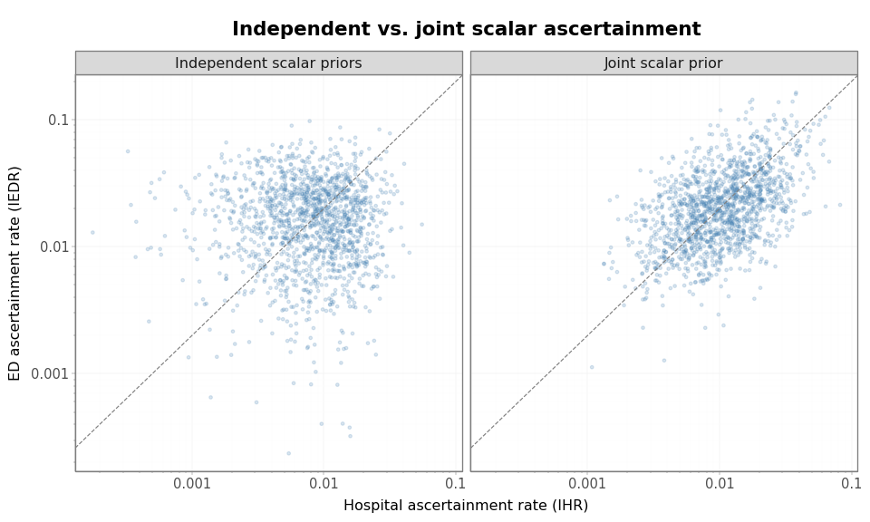
Joint ascertainment induces correlation between scalar signal rates. The dashed line marks the prior-center ratio, IEDR = 2 × IHR. The joint prior keeps the same approximate scale while inducing positive dependence between the two rates.
Using ascertainment with a builder
The main API pattern is:
builder = PyrenewBuilder()
builder.configure_latent(...)

joint_ascertainment = JointAscertainment(
    name="he_ascertainment",
    signals=("hospital", "ed_visits"),
    baseline_rates=jnp.array([0.01, 0.02]),
    scale_tril=jnp.array(
        [
            [0.7, 0.0],
            [0.35, 0.606],
        ]
    ),
)
builder.add_ascertainment(joint_ascertainment)

hospital_obs = PopulationCounts(
    name="hospital",
    ascertainment_rate_rv=joint_ascertainment.for_signal("hospital"),
    delay_distribution_rv=hosp_delay_rv,
    noise=hosp_noise_rv,
    aggregation="weekly",
    reporting_schedule="regular",
    start_dow=MMWR_WEEK,
)
builder.add_observation(hospital_obs)

ed_obs = PopulationCounts(
    name="ed_visits",
    ascertainment_rate_rv=joint_ascertainment.for_signal("ed_visits"),
    delay_distribution_rv=ed_delay_rv,
    noise=ed_noise_rv,
    day_of_week_rv=DeterministicVariable("ed_dow", ed_day_of_week_effects),
)
builder.add_observation(ed_obs)

model = builder.build()
Signal names in for_signal() must match the names used when the
ascertainment model was created. They do not have to match observation
names, but matching them usually makes model code and posterior outputs
easier to read.