Latent Infection Processes

Code

import jax.numpy as jnp
import jax.random as random
import numpy as np
import numpyro
import numpyro.distributions as dist
from numpyro.infer import Predictive
import pandas as pd
import plotnine as p9
import warnings
from plotnine.exceptions import PlotnineWarning

warnings.filterwarnings("ignore", category=PlotnineWarning)

from _tutorial_theme import theme_tutorial

Code

from pyrenew.latent import (
    PopulationInfections,
    AR1,
    DifferencedAR1,
    RandomWalk,
)
from pyrenew.deterministic import DeterministicPMF, DeterministicVariable
from pyrenew.randomvariable import DistributionalVariable

Overview

In infectious disease modeling, the true number of new infections at each time point is not directly observed. Instead, we observe indirect signals: hospital admissions, emergency department visits, reported cases, wastewater concentrations. The latent infection process generates the unobserved infection trajectory that underlies all of these signals.

PyRenew models latent infections using the renewal equation, which describes how new infections arise from recent past infections.

Assume the generation interval has finite support over lags \(\tau = 1, \dots, G\), with

\[\sum_{\tau=1}^{G} w_\tau = 1, \qquad w_\tau \ge 0.\]

Then the renewal equation is

\[I(t) = \mathcal{R}(t) \sum_{\tau=1}^{G} I(t - \tau)\, w_\tau.\]

Here, \(\tau\) indexes lags in the generation interval.

PyRenew provides two latent infection classes:

• PopulationInfections: A single \(\mathcal{R}(t)\) drives one renewal equation. Appropriate when modeling one jurisdiction as a single population with one or more observation streams. This tutorial covers PopulationInfections.
• SubpopulationInfections: A baseline \(\mathcal{R}(t)\) with per-subpopulation deviations. See Latent Subpopulation Infections.

Model Inputs

PopulationInfections requires four inputs:

1. Generation interval distribution \(w_\tau\) (gen_int_rv)
2. Infection prevalence at time \(0\) as a proportion of the population (I0_rv)
3. Value for \(log(\mathcal{R}(t))\) at time \(0\) (log_rt_time_0_rv)
4. A temporal process for \(\mathcal{R}(t)\) dynamics (single_rt_process)

All inputs are RandomVariables, a quantity that is either known (observed, conditioned on) or unknown (to be inferred). See PyRenew’s RandomVariable abstract base class. In this tutorial, we use DeterministicVariable and DeterministicPMF (fixed values) for illustration. In real inference, you would use DistributionalVariable with priors for quantities you want to estimate:

# Fixed value (for illustration)
I0_rv = DeterministicVariable("I0", 0.001)

# With a prior (for inference)
I0_rv = DistributionalVariable("I0", dist.Beta(1, 1000))

Generation Interval

The generation interval is a key epidemiological input to the renewal equation. In many renewal-model analyses, it is specified from external studies rather than estimated jointly from the focal surveillance data. Because R_t estimates depend on this choice, sensitivity analysis is often warranted. For COVID-19, most transmission occurs within the first few days. We define a 7-day distribution for illustration:

Code

gen_int_pmf = jnp.array([0.16, 0.32, 0.25, 0.14, 0.07, 0.04, 0.02])
gen_int_rv = DeterministicPMF("gen_int", gen_int_pmf)

days = np.arange(1, len(gen_int_pmf) + 1)
mean_gi = float(np.sum(days * gen_int_pmf))
print(f"Generation interval: {len(gen_int_pmf)} days, mean = {mean_gi:.1f}")

Generation interval: 7 days, mean = 2.8

Code

gi_df = pd.DataFrame({"day": days, "probability": np.array(gen_int_pmf)})

(
    p9.ggplot(gi_df, p9.aes(x="day", y="probability"))
    + p9.geom_col(fill="steelblue", alpha=0.7, color="black")
    + p9.labs(
        x="Days since primary infection",
        y="Probability",
        title="Generation Interval Distribution",
    )
    + theme_tutorial
)

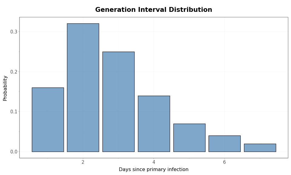
Figure 1: COVID-like generation interval distribution. The support is shown in whole days since infection of the primary case.

The generation interval length determines the minimum initialization period: with a \(G\)-point generation interval distribution, the renewal equation at time \(0\) needs an infection-history vector long enough to supply the previous \(G\) infection values used in the convolution.

Initial Conditions: I0 and log_rt_time_0

These two parameters jointly define the infection history before the observation period begins. Understanding their interaction requires knowing how the latent infections process initializes the renewal equation.

The backprojection mechanism. The renewal equation at time \(0\) needs a vector of recent infections to convolve with the generation interval. The latent infections process constructs this initialization vector via exponential backprojection. Let \(\tau = 0, 1, \ldots, n_{\text{init}} - 1\) index positions in the initialization vector, where \(\tau = 0\) is the earliest time point and \(\tau = n_{\text{init}} - 1\) is the time point immediately before the observation period begins. Then:

\[I_{\text{init}}(\tau) = I_0 \cdot e^{r \cdot \tau}, \quad \tau = 0, 1, \ldots, n_{\text{init}} - 1\]

where \(r\) is the asymptotic growth rate implied by the reproduction number at the start of the observation period, \(\mathcal{R}(t=0) = e^{\text{log\_rt\_time\_0}}\), and the generation interval. The function r_approx_from_R converts \(\mathcal{R}(t=0)\) and the generation interval into \(r\) using Newton’s method.

• The level is set by I0. I0 is the infection prevalence at the earliest point in the initialization period, \(n_{\text{init}} - 1\) time points before \(t = 0\). It sets the scale of the entire initialization vector: \(I_{\text{init}}(0) = I_0\), with subsequent entries growing or declining exponentially toward \(t = 0\).

• The shape is set by log_rt_time_0.
  log_rt_time_0 enters the model in two places: it is the starting point of the \(\mathcal{R}(t)\) trajectory (\(\mathcal{R}(t=0) = e^{\text{log\_rt\_time\_0}}\)), and it determines the exponential growth rate \(r\) used to construct the initialization vector. When log_rt_time_0 = 0, \(r = 0\) and the initialization vector is flat at level I0. When log_rt_time_0 > 0, infections are growing exponentially at \(t = 0\); when log_rt_time_0 < 0, they are declining.

The initialization vector is what the renewal equation “sees” as recent infection history at time \(0\). We can compute it directly for three values of log_rt_time_0:

Code

from pyrenew.math import r_approx_from_R

n_init = len(gen_int_pmf)
I0 = 0.001
init_rt_values = {
    "declining (Rt = 0.82)": -0.2,
    "stable (Rt = 1.0)": 0.0,
    "growing (Rt = 1.22)": 0.2,
}
tau = jnp.arange(n_init)

init_data = []
for label, log_rt in init_rt_values.items():
    Rt0 = jnp.exp(log_rt)
    r = r_approx_from_R(R=Rt0, g=gen_int_pmf, n_newton_steps=4)
    I0_init = I0 * jnp.exp(r * tau)
    for t in range(n_init):
        init_data.append(
            {
                "day": int(t) - n_init,
                "infections": float(I0_init[t]),
                "config": f"log_rt_time_0 = {log_rt} ({label})",
            }
        )
    print(
        f"log_rt_time_0 = {log_rt:+.1f}: Rt(0) = {float(Rt0):.2f}, r = {float(r):.4f}, "
        f"I_init range = [{float(I0_init[0]):.6f}, {float(I0_init[-1]):.6f}]"
    )

init_df = pd.DataFrame(init_data)

log_rt_time_0 = -0.2: Rt(0) = 0.82, r = -0.0687, I_init range = [0.001000, 0.000662]
log_rt_time_0 = +0.0: Rt(0) = 1.00, r = 0.0000, I_init range = [0.001000, 0.001000]
log_rt_time_0 = +0.2: Rt(0) = 1.22, r = 0.0722, I_init range = [0.001000, 0.001543]

Code

(
    p9.ggplot(init_df, p9.aes(x="day", y="infections", color="config"))
    + p9.geom_line(size=1)
    + p9.geom_point(size=2)
    + p9.geom_vline(xintercept=-0.5, linetype="dashed", alpha=0.5)
    + p9.annotate(
        "text", x=-0.3, y=I0 * 1.15, label="day 0 -->", ha="right", size=10
    )
    + p9.labs(
        x="Day (relative to observation start)",
        y="Infections (proportion)",
        title="Initialization Vectors (Exponential Backprojection)",
        color="",
    )
    + theme_tutorial
    + p9.theme(legend_position="bottom", legend_direction="vertical")
)

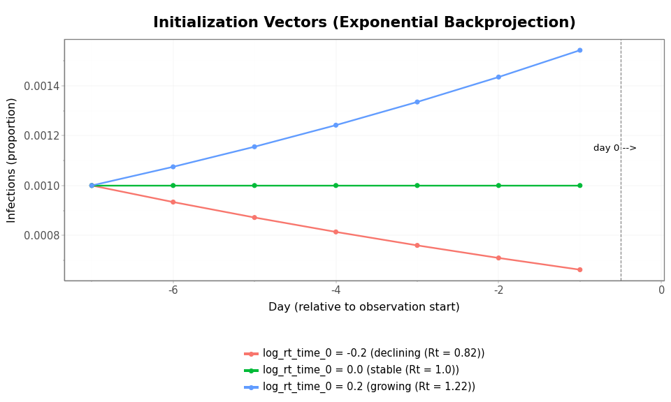
Figure 2: Initialization vectors for three values of log_rt_time_0. Days are numbered relative to day 0, which is when the temporal process and renewal equation take over. When log_rt_time_0 = 0 (stable), the vector is flat. Nonzero values produce exponential growth or decay in the pre-observation period.

The initialization vector matters because the renewal equation is a convolution: infections on day 0 depend on infections from days \(-1\) through \(-(K-1)\), weighted by the generation interval. A flat initialization (stable) means the renewal equation starts with uniform recent history. A growing initialization means the most recent days have disproportionately more infections, which amplifies the effect of the generation interval’s short-lag weights.

After day 0, the temporal process takes over. How quickly the trajectory departs from its initial behavior depends on the temporal process choice and its hyperparameters, which we examine in the next section.

Temporal Process Choice

The temporal process governs how \(\log \mathcal{R}(t)\) evolves day to day.

To evaluate what a given process implies, we use prior predictive checks: drawing many samples from the model before seeing any data and examining the distribution of trajectories. A single sample tells you little (the trajectory depends on the random seed), but the envelope of many samples reveals the structural constraints built into the process. We fix the initial conditions to a growing epidemic (log_rt_time_0 = 0.5, so \(\mathcal{R}(0) \approx 1.65\)) with I0 = 0.001. Starting well above equilibrium rather than near it makes the behavioral differences between temporal processes visible: the median trajectory of a mean-reverting process drifts back toward \(\mathcal{R} = 1\), while a non-reverting process does not.

This section is primarily modeling guidance for prior specification in PyRenew, not a claim that epidemiologic theory uniquely determines one temporal process choice. The appropriate process depends on the scientific setting, time horizon, and how strongly you want the prior to regularize latent transmission dynamics.

Code

n_days = 28
n_init = len(gen_int_pmf)
n_samples = 200
log_rt_time_0 = 0.5
I0_val = 0.001
rt_cap = 3.0


def sample_process(rt_process, label):
    """Draw prior predictive samples for a given temporal process."""
    model = PopulationInfections(
        name="PopulationInfections",
        gen_int_rv=gen_int_rv,
        I0_rv=DeterministicVariable("I0", I0_val),
        log_rt_time_0_rv=DeterministicVariable("log_rt_time_0", log_rt_time_0),
        single_rt_process=rt_process,
        n_initialization_points=n_init,
    )

    def sampler():
        """Wrapper for Predictive."""
        return model.sample(n_days_post_init=n_days)

    samples = Predictive(sampler, num_samples=n_samples)(random.PRNGKey(42))
    return {
        "rt": np.array(samples["PopulationInfections::rt_single"])[
            :, n_init:, 0
        ],
        "infections": np.array(
            samples["PopulationInfections::infections_aggregate"]
        )[:, n_init:],
    }


def rt_spaghetti_plot(rt_array, title, color="steelblue"):
    """Build a spaghetti plot of Rt trajectories with a median + 90% ribbon overlay."""
    n_traj, n_t = rt_array.shape
    spaghetti_data = []
    for i in range(n_traj):
        for d in range(n_t):
            spaghetti_data.append(
                {"day": d, "rt": float(rt_array[i, d]), "sample": i}
            )
    df = pd.DataFrame(spaghetti_data)
    summary_df = pd.DataFrame(
        {
            "day": np.arange(n_t),
            "median": np.median(rt_array, axis=0),
            "q05": np.percentile(rt_array, 5, axis=0),
            "q95": np.percentile(rt_array, 95, axis=0),
        }
    )
    return (
        p9.ggplot()
        + p9.geom_line(
            df,
            p9.aes(x="day", y="rt", group="sample"),
            alpha=0.08,
            size=0.5,
            color=color,
        )
        + p9.geom_ribbon(
            summary_df,
            p9.aes(x="day", ymin="q05", ymax="q95"),
            fill=color,
            alpha=0.25,
        )
        + p9.geom_line(
            summary_df,
            p9.aes(x="day", y="median"),
            color=color,
            size=1.0,
        )
        + p9.geom_hline(
            yintercept=1.0, color="red", linetype="dashed", alpha=0.7
        )
        + p9.coord_cartesian(ylim=(0, rt_cap))
        + p9.labs(x="Days", y="Rt", title=title)
        + theme_tutorial
    )


def rt_summary(rt_array, label):
    """Print summary statistics for Rt at the final time point."""
    rt_final = rt_array[:, -1]
    n_above_cap = np.sum(np.any(rt_array > rt_cap, axis=1))
    print(f"{label}:")
    print(
        f"  Rt at day {rt_array.shape[1]}:  "
        f"median = {np.median(rt_final):.2f}, "
        f"90% interval = [{np.percentile(rt_final, 5):.2f}, {np.percentile(rt_final, 95):.2f}], "
        f"max = {np.max(rt_final):.1f}"
    )
    if n_above_cap > 0:
        print(
            f"  {n_above_cap} of {rt_array.shape[0]} samples exceed Rt = {rt_cap} "
            f"(clipped in plot)"
        )

Random Walk

The simplest temporal process.

\[x_t = x_{t-1} + \varepsilon_t, \quad \varepsilon_t \sim N(0, \sigma)\]

There is no tendency to return to any particular value. Once \(\mathcal{R}(t)\) drifts up or down, it stays there until noise pushes it elsewhere. The variance of \(x_t\) grows linearly with time: \(\text{Var}(x_t) = \sigma^2 t\). The further into the future, the less constrained the process is.

Hyperparameter: innovation_sd (\(\sigma\)) is the standard deviation of each daily step on the log scale. With innovation_sd = 0.05, each day’s \(\log \mathcal{R}\) changes by roughly \(\pm 0.05\), which corresponds to roughly \(\pm 5\%\) multiplicative change in \(\mathcal{R}\).

Code

rw_samples = sample_process(RandomWalk(innovation_sd=0.05), "RandomWalk")

Code

rt_spaghetti_plot(rw_samples["rt"], "Random Walk (innovation_sd = 0.05)")

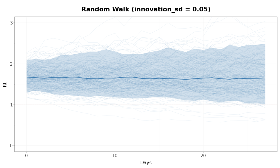
Figure 3: Prior predictive \(\mathcal{R}(t)\) trajectories under a Random Walk (innovation_sd = 0.05). The envelope widens steadily over time because variance grows linearly. Trajectories drift in both directions from the starting value with no tendency to return.

Code

rt_summary(rw_samples["rt"], "Random Walk (innovation_sd = 0.05)")

Random Walk (innovation_sd = 0.05):
  Rt at day 28:  median = 1.63, 90% interval = [1.01, 2.48], max = 3.7
  4 of 200 samples exceed Rt = 3.0 (clipped in plot)

AR(1)

An autoregressive process of order 1. Each day, \(\log \mathcal{R}(t)\) is pulled toward zero (i.e., \(\mathcal{R} = 1\)) by the autoregressive coefficient \(\phi\):

\[x_t = \phi \, x_{t-1} + \varepsilon_t, \quad \varepsilon_t \sim N(0, \sigma)\]

When \(|\phi| < 1\), the process is stationary: its variance does not grow with time but is bounded at \(\sigma^2 / (1 - \phi^2)\). This means the process “forgets” its initial value and fluctuates within a stable envelope. If \(\mathcal{R}(t)\) drifts above 1, the \(\phi\) coefficient pulls it back; if it drifts below, it pulls it up.

Hyperparameters:

• autoreg (\(\phi\)): controls the strength and speed of mean reversion. Values near 1 produce slow reversion (the process remembers its recent past); values near 0 produce fast reversion (the process snaps back quickly).
• innovation_sd (\(\sigma\)): standard deviation of daily noise.

The two hyperparameters jointly determine the stationary standard deviation \(\sigma_{\text{stat}} = \sigma / \sqrt{1 - \phi^2}\), which is the long-run spread of \(\log \mathcal{R}(t)\). For example, autoreg = 0.9 and innovation_sd = 0.05 give \(\sigma_{\text{stat}} \approx 0.115\), meaning 95% of long-run \(\log \mathcal{R}\) values fall within \(\pm 0.23\) of zero, or equivalently \(\mathcal{R} \in [0.79, 1.26]\).

Code

ar1_samples = sample_process(AR1(autoreg=0.9, innovation_sd=0.05), "AR1")

Code

rt_spaghetti_plot(
    ar1_samples["rt"], "AR(1) (autoreg = 0.9, innovation_sd = 0.05)"
)

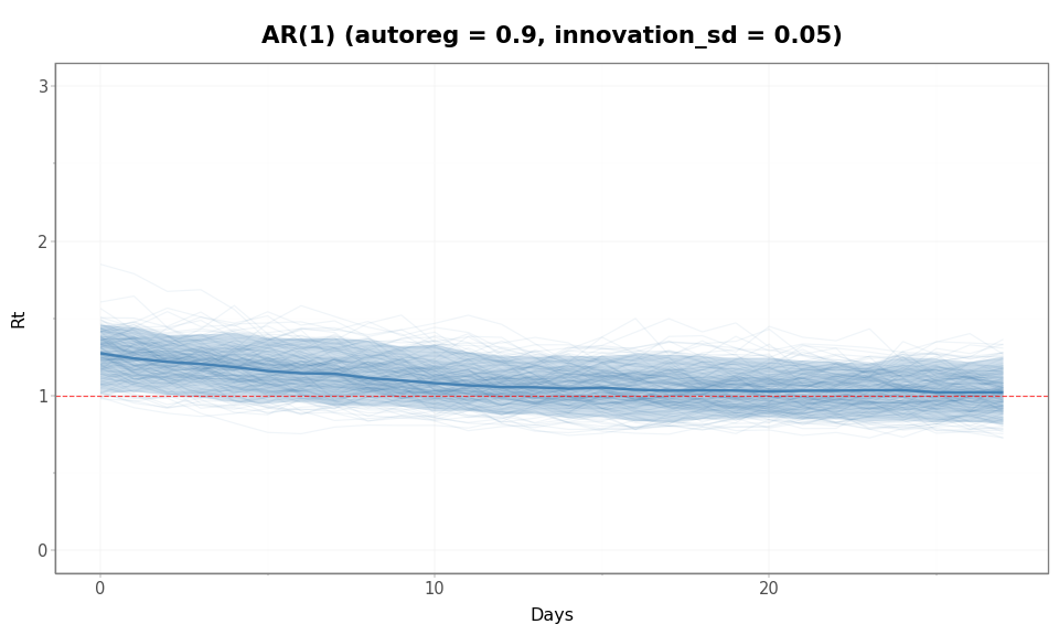
Figure 4: Prior predictive \(\mathcal{R}(t)\) trajectories under AR(1) (autoreg = 0.9, innovation_sd = 0.05). The envelope stabilizes rather than growing over time. The median trajectory (solid line) drifts from the starting \(\mathcal{R}(0)\) of 1.65 back toward 1, illustrating mean reversion of the level.

Code

rt_summary(ar1_samples["rt"], "AR(1) (autoreg = 0.9, innovation_sd = 0.05)")

AR(1) (autoreg = 0.9, innovation_sd = 0.05):
  Rt at day 28:  median = 1.02, 90% interval = [0.81, 1.25], max = 1.4

DifferencedAR1

DifferencedAR1 models changes in \(\mathcal{R}(t)\) as an autoregressive process. In terms of increments,

\[\Delta x_t = \texttt{autoreg} \cdot \Delta x_{t-1} + \varepsilon_t, \quad x_t = x_{t-1} + \Delta x_t,\]

so the autoregressive structure applies to the rate of change rather than the level.

This has an important consequence: while changes in \(\mathcal{R}(t)\) are mean-reverting, the level itself is not. As a result, trajectories can exhibit sustained upward or downward trends and may drift over time, even when the innovations are small. This process accumulates changes over time, so variability builds up in the level. Because successive changes are correlated, increases or decreases can persist for several steps in a row. These sustained runs can lead to wider trajectories than a random walk with the same innovation_sd, even though the individual innovations are small.

Hyperparameters:

• autoreg (\(\phi\)): controls persistence of the rate of change. Values near 1 mean trends persist longer; values near 0 mean trends dissipate quickly.
• innovation_sd (\(\sigma\)): standard deviation of shocks to the rate of change (not to the level).

We use innovation_sd = 0.01 (smaller than the 0.05 used for Random Walk and AR(1) above).

Code

dar1_samples = sample_process(
    DifferencedAR1(autoreg=0.5, innovation_sd=0.01), "DifferencedAR1"
)

Code

rt_spaghetti_plot(
    dar1_samples["rt"],
    "DifferencedAR1 (autoreg = 0.5, innovation_sd = 0.01)",
)

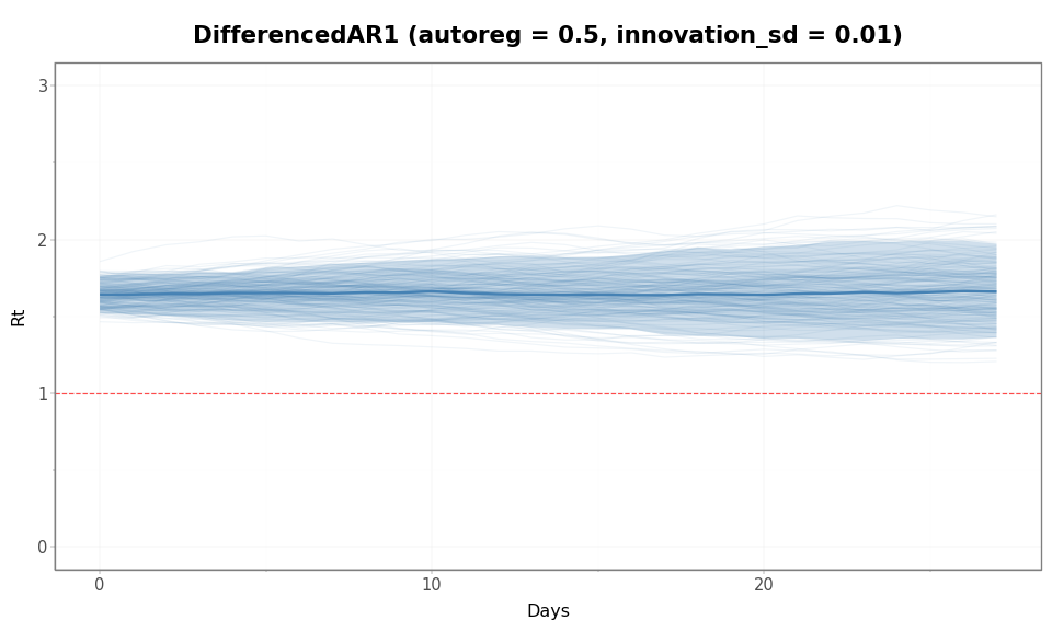
Figure 5: DifferencedAR1 allows sustained directional trends because the increments are autocorrelated. Even with a smaller innovation scale than the other examples, the induced prior on \(\mathcal{R}(t)\) can still be fairly diffuse over this time horizon.

Code

rt_summary(
    dar1_samples["rt"], "DifferencedAR1 (autoreg = 0.5, innovation_sd = 0.01)"
)

DifferencedAR1 (autoreg = 0.5, innovation_sd = 0.01):
  Rt at day 28:  median = 1.66, 90% interval = [1.36, 1.97], max = 2.2

Comparing the Three Processes

The plots above use different hyperparameter values for each process. This is intentional: the parameters innovation_sd and autoreg play different roles across processes (daily step size for RandomWalk, noise around the level for AR(1), and shocks to the rate of change for DifferencedAR1), so equal numerical values are not directly comparable.

For AR(1), autoreg controls how strongly \(\mathcal{R}(t)\) is pulled back toward \(1\), directly limiting variation in the level. For DifferencedAR1, autoreg instead controls how persistent changes are over time. Because these changes accumulate, even small innovations can produce substantial drift in \(\mathcal{R}(t)\) when persistence is high.

As a result, DifferencedAR1 can exhibit wider trajectories than might be expected from the scale of innovation_sd alone. Hyperparameters are chosen to illustrate characteristic behavior rather than to match marginal variability, so the resulting spreads are not directly comparable across panels.

Code

comparison_data = []
process_labels = {
    "Random Walk\n(sd=0.05)": rw_samples,
    "AR(1)\n(autoreg=0.9, sd=0.05)": ar1_samples,
    "DifferencedAR1\n(autoreg=0.5, sd=0.01)": dar1_samples,
}
for label, s in process_labels.items():
    rt = s["rt"]
    for i in range(n_samples):
        for d in range(n_days):
            comparison_data.append(
                {
                    "day": d,
                    "rt": float(rt[i, d]),
                    "sample": i,
                    "process": label,
                }
            )
comparison_df = pd.DataFrame(comparison_data)
comparison_df["process"] = pd.Categorical(
    comparison_df["process"],
    categories=list(process_labels.keys()),
    ordered=True,
)

Code

(
    p9.ggplot(
        comparison_df.groupby(["process", "day"])["rt"]
        .agg(
            q05=lambda x: np.percentile(x, 5),
            median="median",
            q95=lambda x: np.percentile(x, 95),
        )
        .reset_index(),
        p9.aes(x="day"),
    )
    + p9.geom_ribbon(
        p9.aes(ymin="q05", ymax="q95"),
        fill="steelblue",
        alpha=0.2,
    )
    + p9.geom_line(
        p9.aes(y="median"),
        color="steelblue",
        size=1.0,
    )
    + p9.geom_hline(yintercept=1.0, color="red", linetype="dashed", alpha=0.7)
    + p9.facet_wrap("~ process", ncol=3)
    + p9.coord_cartesian(ylim=(0, rt_cap))
    + p9.labs(x="Days", y="Rt", title="Temporal Process Comparison")
    + theme_tutorial
)

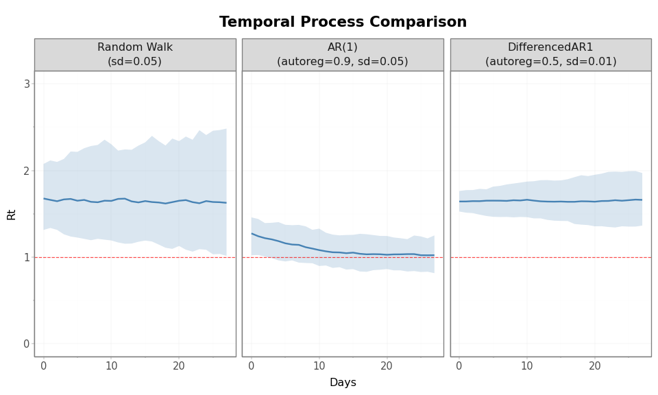
Figure 6: Side-by-side comparison of all three temporal processes using median trajectories and 90% prior intervals.

Code

summary_rows = []
for label, ar, sd, s in [
    ("Random Walk", None, 0.05, rw_samples),
    ("AR(1)", 0.9, 0.05, ar1_samples),
    ("DifferencedAR1", 0.5, 0.01, dar1_samples),
]:
    rt = s["rt"][:, -1]
    summary_rows.append(
        {
            "Process": label,
            "autoreg": "-" if ar is None else f"{ar:.2f}",
            "innovation_sd": f"{sd:.2f}",
            "Median": f"{np.median(rt):.2f}",
            "5%": f"{np.percentile(rt, 5):.2f}",
            "95%": f"{np.percentile(rt, 95):.2f}",
            "Max": f"{np.max(rt):.1f}",
        }
    )
pd.DataFrame(summary_rows)

Table 1: \(\mathcal{R}(t)\) at day 28 by temporal process.

	Process	autoreg	innovation_sd	Median	5%	95%	Max
0	Random Walk	-	0.05	1.63	1.01	2.48	3.7
1	AR(1)	0.90	0.05	1.02	0.81	1.25	1.4
2	DifferencedAR1	0.50	0.01	1.66	1.36	1.97	2.2

When to use which process:

• AR(1) assumes \(\mathcal{R}(t)\) reverts to \(1\). Appropriate when modeling a pathogen near endemic equilibrium, or over short time horizons where large sustained departures from the current level are implausible.
• Random Walk assumes no preferred direction and no memory beyond the current value. Appropriate when you have little prior knowledge about whether \(\mathcal{R}(t)\) will increase or decrease, and the data are dense enough to constrain the trajectory.
• DifferencedAR1 assumes trends can persist but the rate of change stabilizes. Appropriate for epidemic waves where \(\mathcal{R}(t)\) can sustain a direction of movement (e.g., rising during a wave, declining after interventions).

Effect of Hyperparameters

The hyperparameters autoreg and innovation_sd control how tightly the prior constrains \(\mathcal{R}(t)\), but their roles differ in important ways for DifferencedAR1.

The innovation_sd parameter sets the scale of shocks to the rate of change in \(\mathcal{R}(t)\), while autoreg controls how persistent those changes are over time. In terms of increments, where \(\phi =\) autoreg

\[\Delta x_t = \phi \cdot \Delta x_{t-1} + \varepsilon_t\]

autoreg (\(\phi\)) determines how strongly each change carries forward into the next. The level then accumulates these changes via \(x_t = x_{t-1} + \Delta x_t\).

When autoreg is large (e.g., 0.9), increments are highly persistent: a positive change in \(\mathcal{R}(t)\) is likely to be followed by further positive changes. This produces sustained upward or downward trends, even when innovation_sd is small. Because these persistent changes accumulate in the level, the resulting prior over \(\mathcal{R}(t)\) can be relatively diffuse over time.

Lowering autoreg reduces this persistence. Increments decorrelate more quickly, causing positive and negative changes to cancel out, which limits long runs of same-direction movement and produces a tighter prior over \(\mathcal{R}(t)\).

Importantly, this differs from AR(1): in AR(1), autoreg controls mean reversion of the level, directly shrinking \(\mathcal{R}(t)\) toward its mean. In DifferencedAR1, only the changes are mean-reverting, so the level itself can drift. As a result, controlling long-term variability in DifferencedAR1 typically requires adjusting both innovation_sd (step size) and autoreg (persistence of trends).

We illustrate these effects below for DifferencedAR1 by varying both parameters:

Code

hyperparam_configs = {
    "autoreg=0.5, sd=0.01": DifferencedAR1(autoreg=0.5, innovation_sd=0.01),
    "autoreg=0.9, sd=0.02": DifferencedAR1(autoreg=0.9, innovation_sd=0.02),
    "autoreg=0.95, sd=0.05": DifferencedAR1(autoreg=0.95, innovation_sd=0.05),
}

hyperparam_samples = {}
for name, rt_process in hyperparam_configs.items():
    hyperparam_samples[name] = sample_process(rt_process, name)

Code

hp_data = []
for name in hyperparam_configs:
    rt = hyperparam_samples[name]["rt"]
    for i in range(n_samples):
        for d in range(n_days):
            hp_data.append(
                {"day": d, "rt": float(rt[i, d]), "sample": i, "config": name}
            )
hp_df = pd.DataFrame(hp_data)
hp_df["config"] = pd.Categorical(
    hp_df["config"],
    categories=list(hyperparam_configs.keys()),
    ordered=True,
)

Code

(
    p9.ggplot(hp_df, p9.aes(x="day", y="rt", group="sample"))
    + p9.geom_line(alpha=0.1, size=0.5, color="steelblue")
    + p9.geom_hline(yintercept=1.0, color="red", linetype="dashed", alpha=0.7)
    + p9.facet_wrap("~ config", ncol=3)
    + p9.coord_cartesian(ylim=(0, rt_cap))
    + p9.labs(
        x="Days",
        y="Rt",
        title=r"DifferencedAR1: Effect of Hyperparameters on Prior $\mathcal{R}(t)$",
    )
    + theme_tutorial
)

Figure 7: Effect of DifferencedAR1 hyperparameters on prior \(\mathcal{R}(t)\) distribution. Lower autoreg and innovation_sd (left) produce a tighter envelope; higher values (right) allow wider drift. All start at \(\mathcal{R}(0)\) = 1.65.

Code

hp_summary_rows = []
for name in hyperparam_configs:
    rt = hyperparam_samples[name]["rt"][:, -1]
    hp_summary_rows.append(
        {
            "Config": name,
            "Median": f"{np.median(rt):.2f}",
            "5%": f"{np.percentile(rt, 5):.2f}",
            "95%": f"{np.percentile(rt, 95):.2f}",
        }
    )
pd.DataFrame(hp_summary_rows)

Table 2: \(\mathcal{R}(t)\) at day 28 by DifferencedAR1 configuration.

	Config	Median	5%	95%
0	autoreg=0.5, sd=0.01	1.66	1.36	1.97
1	autoreg=0.9, sd=0.02	1.52	0.30	7.32
2	autoreg=0.95, sd=0.05	1.21	0.00	672.53

Both hyperparameters matter, and they interact:

• Lower autoreg means faster reversion of the rate of change toward zero, producing trajectories that settle more quickly.
• Lower innovation_sd means smaller daily shocks to the rate of change, producing smoother trends.

There are no universally correct hyperparameter values. The right choice depends on the pathogen, the time horizon, and the density of the available data. Prior predictive checks are the tool for evaluating whether a given configuration produces trajectories that are scientifically plausible for your setting.

Infection Trajectories

\(\mathcal{R}(t)\) drives the renewal equation, but the infection trajectory \(I(t)\) is what observation processes actually transform into data. The transformation from \(\mathcal{R}(t)\) to \(I(t)\) is nonlinear (growth compounds exponentially), so the distribution of infection trajectories has heavier tails and stronger skew than the distribution of \(\mathcal{R}(t)\).

Code

inf_comparison = []
for label, s in process_labels.items():
    inf = s["infections"]
    for i in range(n_samples):
        for d in range(n_days):
            inf_comparison.append(
                {
                    "day": d,
                    "infections": float(inf[i, d]),
                    "sample": i,
                    "process": label,
                }
            )
inf_comparison_df = pd.DataFrame(inf_comparison)
inf_comparison_df["process"] = pd.Categorical(
    inf_comparison_df["process"],
    categories=list(process_labels.keys()),
    ordered=True,
)

Code

(
    p9.ggplot(
        inf_comparison_df, p9.aes(x="day", y="infections", group="sample")
    )
    + p9.geom_line(alpha=0.1, size=0.4, color="darkorange")
    + p9.facet_wrap("~ process", ncol=3)
    + p9.scale_y_log10()
    + p9.labs(
        x="Days",
        y="Infections (proportion, log scale)",
        title="Prior Predictive: Infection Trajectories by Temporal Process",
    )
    + theme_tutorial
)

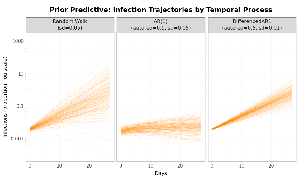
Figure 8: Prior predictive infection trajectories (log scale). The nonlinear transformation from \(\mathcal{R}(t)\) to infections amplifies differences between temporal processes. The vertical spread represents orders-of-magnitude differences in infection levels.

Connecting to Observation Processes

The latent infection trajectory is not observed directly. To connect it to data, one or more observation processes transform \(I(t)\) into expected observations.

The PyrenewBuilder handles the wiring:

1. configure_latent() sets the single infection process (called once)
2. add_observation() adds an observation process (called once per data stream)
3. build() computes n_initialization_points from all delay distributions and produces a model ready for inference

To learn how to build complete models with observation processes, see:

• Observation Processes: Counts
• Observation Processes: Measurements
• Building Multi-Signal Models