Observation processes for continuous measurements
This tutorial demonstrates how to use the MeasurementObservation
observation process to model continuous measurement data. We first
explain the general framework, then illustrate with a wastewater viral
concentration example.
Code
import jax
import jax.numpy as jnp
import numpy as np
import numpyro
import pandas as pd
import plotnine as p9

import numpyro.distributions as dist
from _tutorial_theme import theme_tutorial

from pyrenew.observation import (
    MeasurementObservation,
    HierarchicalNormalNoise,
)
from pyrenew.randomvariable import DistributionalVariable, VectorizedVariable
from pyrenew.deterministic import DeterministicVariable, DeterministicPMF
The MeasurementObservation Class
The MeasurementObservation class models continuous signals derived
from infections. Unlike count observations (hospital admissions,
deaths), measurements are continuous values that may span orders of
magnitude or even be negative (e.g., log-transformed data).
Examples of measurement data:
- Wastewater viral concentrations
- Air quality pathogen levels
- Serological assay results
- Environmental sensor readings
The general pattern
All measurement observation processes follow the same two-layer structure as the count observation model:
- A deterministic transformation defining the expected measurement value
- A stochastic observation model
Let \(\mu(t)\) denote the expected measurement at time \(t\). Observations are modeled as
where \(f(\cdot)\) is a transformation (often the identity or log function), and the noise model adds stochastic variation around this transformed prediction.
Subclasses implement _predicted_obs() to compute \(\mu(t)\) from
infections. PyRenew provides the noise model.
The MeasurementObservation base class provides:
- Convolution utilities for temporal delays
- Timeline alignment between infections and observations
- Integration with hierarchical noise models
- Support for multiple sensors and subpopulations
Comparison with count observations
The core convolution structure is shared with count observations, but key aspects differ:
| Aspect | CountObservation | MeasurementObservation |
|---|---|---|
| Output type | Discrete counts | Continuous values |
| Output space | Linear (expected counts) | Often log-transformed |
| Noise model | Poisson or Negative Binomial | Normal (often on log scale) |
| Scaling | Ascertainment rate \(\alpha \in [0,1]\) | Domain-specific |
| Subpop structure | Optional (CountsBySubpop) |
Inherent (sensor/site effects) |
The noise model
Measurement data typically exhibits sensor-level variability: different instruments, labs, or sampling locations may have systematic biases and different precision levels.
HierarchicalNormalNoise models this with two per-sensor parameters:
- Sensor mode: Systematic bias (additive shift)
- Sensor SD: Measurement precision (noise level)
observed ~ Normal(f(\mu(t)) + sensor_mode[sensor], sensor_sd[sensor])
The sensor-level RVs must implement sample(n_groups=...). Use
VectorizedVariable to wrap simple distributions:
Code
# Sensor modes: zero-centered, allowing positive or negative bias
sensor_mode_rv = VectorizedVariable(
    "vec_sensor_mode",
    DistributionalVariable("sensor_mode", dist.Normal(0, 0.5)),
)

# Sensor SDs: must be positive, truncated normal is a common choice
sensor_sd_rv = VectorizedVariable(
    "vec_sensor_sd",
    DistributionalVariable(
        "sensor_sd", dist.TruncatedNormal(loc=0.3, scale=0.15, low=0.05)
    ),
)

# Create noise model
noise = HierarchicalNormalNoise(
    sensor_mode_rv=sensor_mode_rv,
    sensor_sd_rv=sensor_sd_rv,
)
The indexing system
Measurement observations use three index arrays to map observations to their context:
| Index array | Purpose |
|---|---|
times |
Day index for each observation |
subpop_indices |
Which infection trajectory (subpopulation) generated each observation |
sensor_indices |
Which sensor made each observation (determines noise parameters) |
This flexible indexing supports:
- Irregular sampling: Observations don’t need to be daily
- Multiple sensors per subpopulation: Different labs analyzing the same source
- Multiple subpopulations per sensor: One sensor serving multiple areas (less common)
Subclassing MeasurementObservation
To create a measurement process for your domain, subclass
MeasurementObservation and implement:
_predicted_obs(infections): Transform infections to predicted valuesvalidate(): Check parameter validitylookback_days(): Return the temporal PMF length
The MeasurementObservation base class requires a name parameter.
Observation processes are components in multi-signal models, where each
signal must have a unique, meaningful name (e.g., "wastewater",
"air_quality"). This name prefixes all numpyro sample sites, ensuring
distinct identifiers in the inference trace.
class MyMeasurement(MeasurementObservation):
    def __init__(self, name, temporal_pmf_rv, noise, my_scaling_param):
        super().__init__(name=name, temporal_pmf_rv=temporal_pmf_rv, noise=noise)
        self.my_scaling_param = my_scaling_param

    def _predicted_obs(self, infections):
        # Your domain-specific transformation here
        pmf = self.temporal_pmf_rv()
        # ... convolve, scale, transform ...
        return predicted_values

    def validate(self):
        pmf = self.temporal_pmf_rv()
        self._validate_pmf(pmf, "temporal_pmf_rv")

    def lookback_days(self):
        return len(self.temporal_pmf_rv()) - 1
Measurement Example: Wastewater
To illustrate the framework, we specify a wastewater viral concentration observation process, based on the PyRenew-HEW family of models.
The wastewater signal
Wastewater treatment plants measure viral RNA concentrations in sewage. The concentration is determined by:
- Infections: People shed virus into wastewater
- Shedding kinetics: Viral shedding peaks a few days after infection
- Scaling factors: Genome copies per infection and wastewater volume
Observation model
The predicted concentration at time \(t\) is given by
where:
- \(I(t-d)\) is the number of infections on day \(t-d\)
- \(\pi_d\) is the shedding kinetics PMF, giving the fraction of total shedding occurring \(d\) days after infection, analogous to the delay distribution in count observation models
- \(G\) is the number of genome copies shed per infection
- \(V\) is the wastewater volume per person per day
This has the same convolution structure as the observation equation for count data, with a different transformation applied to the expected value.
We model the observed log-concentration as
where:
- \(Y(t)\) is the observed log-concentration at time \(t\)
- \(\text{sensor\_mode}\) represents a sensor-specific bias (additive shift on the log scale)
- \(\text{sensor\_sd}\) represents the measurement variability for that sensor
Interpretation
This model follows the same two-layer structure used for count observations:
- A deterministic layer, where the convolution defines the predicted concentration \(\mu(t)\) from latent infections
- A stochastic observation layer, where observed measurements \(Y(t)\) vary around \(\log(\mu(t))\) due to sensor noise
The key difference from count data is that measurements are modeled on a continuous (often log-transformed) scale, and variability is represented using a normal distribution rather than a count distribution.
Implementing the Wastewater class
Code
from jax.typing import ArrayLike
from pyrenew.metaclass import RandomVariable
from pyrenew.observation.noise import MeasurementNoise


class Wastewater(MeasurementObservation):
    """
    Wastewater viral concentration observation process.

    Transforms site-level infections into predicted log-concentrations
    via shedding kinetics convolution and genome/volume scaling.
    """

    def __init__(
        self,
        name: str,
        shedding_kinetics_rv: RandomVariable,
        log10_genome_per_infection_rv: RandomVariable,
        ml_per_person_per_day: float,
        noise: MeasurementNoise,
    ) -> None:
        """
        Initialize wastewater observation process.

        Parameters
        ----------
        name : str
            Unique name for this observation process.
        shedding_kinetics_rv : RandomVariable
            Viral shedding PMF (fraction shed each day post-infection).
        log10_genome_per_infection_rv : RandomVariable
            Log10 genome copies shed per infection.
        ml_per_person_per_day : float
            Wastewater volume per person per day (mL).
        noise : MeasurementNoise
            Noise model (e.g., HierarchicalNormalNoise).
        """
        super().__init__(name=name, temporal_pmf_rv=shedding_kinetics_rv, noise=noise)
        self.log10_genome_per_infection_rv = log10_genome_per_infection_rv
        self.ml_per_person_per_day = ml_per_person_per_day

    def validate(self) -> None:
        """Validate parameters."""
        shedding_pmf = self.temporal_pmf_rv()
        self._validate_pmf(shedding_pmf, "shedding_kinetics_rv")
        self.noise.validate()

    def lookback_days(self) -> int:
        """Return required lookback (PMF length minus 1)."""
        return len(self.temporal_pmf_rv()) - 1

    def _predicted_obs(self, infections: ArrayLike) -> ArrayLike:
        """
        Compute the log of the expected concentration from infections.
        This corresponds to log(mu(t)), where mu(t) is defined by the observation equation.
        Applies shedding kinetics convolution, then scales by
        genome copies and volume to get concentration.
        """
        shedding_pmf = self.temporal_pmf_rv()
        log10_genome = self.log10_genome_per_infection_rv()

        # Convolve each site's infections with shedding kinetics
        def convolve_site(site_infections):
            convolved, _ = self._convolve_with_alignment(
                site_infections, shedding_pmf, p_observed=1.0
            )
            return convolved

        # Apply to all subpops (infections shape: n_days x n_subpops)
        shedding_signal = jax.vmap(convolve_site, in_axes=1, out_axes=1)(infections)

        # Convert to concentration: genomes per mL
        genome_copies = 10**log10_genome
        concentration = shedding_signal * genome_copies / self.ml_per_person_per_day

        # Return log-concentration (what we model)
        return jnp.log(concentration)
Configuring wastewater-specific parameters
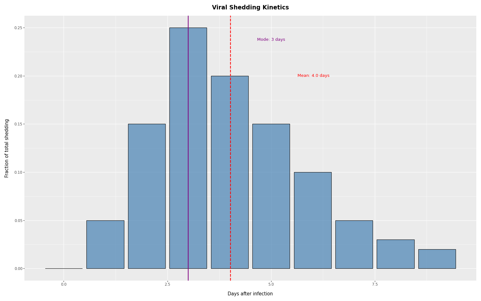
Viral shedding kinetics
The shedding PMF describes what fraction of total viral shedding occurs on each day after infection:
Code
# Peak shedding ~3 days after infection, continues for ~10 days
shedding_pmf = jnp.array([0.0, 0.05, 0.15, 0.25, 0.20, 0.15, 0.10, 0.05, 0.03, 0.02])
print(f"PMF sums to: {shedding_pmf.sum():.2f}")

shedding_rv = DeterministicPMF("viral_shedding", shedding_pmf)

# Summary statistics
days = np.arange(len(shedding_pmf))
mean_shedding_day = float(np.sum(days * shedding_pmf))
mode_shedding_day = int(np.argmax(shedding_pmf))
print(f"Mode: {mode_shedding_day} days, Mean: {mean_shedding_day:.1f} days")
PMF sums to: 1.00
Mode: 3 days, Mean: 4.0 days
Code
# Visualize the shedding distribution
shedding_df = pd.DataFrame({"days": days, "probability": np.array(shedding_pmf)})

(
    p9.ggplot(shedding_df, p9.aes(x="days", y="probability"))
    + p9.geom_col(fill="steelblue", alpha=0.7, color="black")
    + p9.geom_vline(
        xintercept=mode_shedding_day, color="purple", linetype="solid", size=1
    )
    + p9.geom_vline(
        xintercept=mean_shedding_day, color="red", linetype="dashed", size=1
    )
    + p9.labs(
        x="Days after infection",
        y="Fraction of total shedding",
        title="Viral Shedding Kinetics",
    )
    + theme_tutorial
    + p9.annotate(
        "text",
        x=mode_shedding_day + 2,
        y=max(shedding_df["probability"]) * 0.95,
        label=f"Mode: {mode_shedding_day} days",
        color="purple",
        size=10,
    )
    + p9.annotate(
        "text",
        x=mean_shedding_day + 2,
        y=max(shedding_df["probability"]) * 0.8,
        label=f"Mean: {mean_shedding_day:.1f} days",
        color="red",
        size=10,
    )
)
Genome copies and wastewater volume
Code
# Log10 genome copies shed per infection (typical range: 8-10)
log10_genome_rv = DeterministicVariable("log10_genome", 9.0)

# Wastewater volume per person per day (mL)
ml_per_person_per_day = 1000.0
Sensor-level noise
For wastewater, a “sensor” is a WWTP/lab pair—the combination of treatment plant and laboratory that determines measurement characteristics:
Code
# Sensor-level mode: systematic differences between WWTP/lab pairs
ww_sensor_mode_rv = VectorizedVariable(
    "vec_ww_sensor_mode",
    DistributionalVariable("ww_sensor_mode", dist.Normal(0, 0.5)),
)

# Sensor-level SD: measurement variability within each WWTP/lab pair
ww_sensor_sd_rv = VectorizedVariable(
    "vec_ww_sensor_sd",
    DistributionalVariable(
        "ww_sensor_sd", dist.TruncatedNormal(loc=0.3, scale=0.15, low=0.10)
    ),
)

ww_noise = HierarchicalNormalNoise(
    sensor_mode_rv=ww_sensor_mode_rv,
    sensor_sd_rv=ww_sensor_sd_rv,
)
Creating the wastewater observation process
Code
ww_process = Wastewater(
    name="wastewater",
    shedding_kinetics_rv=shedding_rv,
    log10_genome_per_infection_rv=log10_genome_rv,
    ml_per_person_per_day=ml_per_person_per_day,
    noise=ww_noise,
)

print(f"Required lookback: {ww_process.lookback_days()} days")
Required lookback: 9 days
Simulations
Timeline alignment
The observation process maintains alignment: day \(t\) in output
corresponds to day \(t\) in input. A temporal PMF of length \(L\) covers
lags 0 to \(L-1\), requiring \(L-1\) days of prior history. The method
lookback_days() returns \(L-1\); the first valid observation day is at
index lookback_days().
Code
def first_valid_observation_day(obs_process) -> int:
    """Return the first day index with complete infection history."""
    return obs_process.lookback_days()
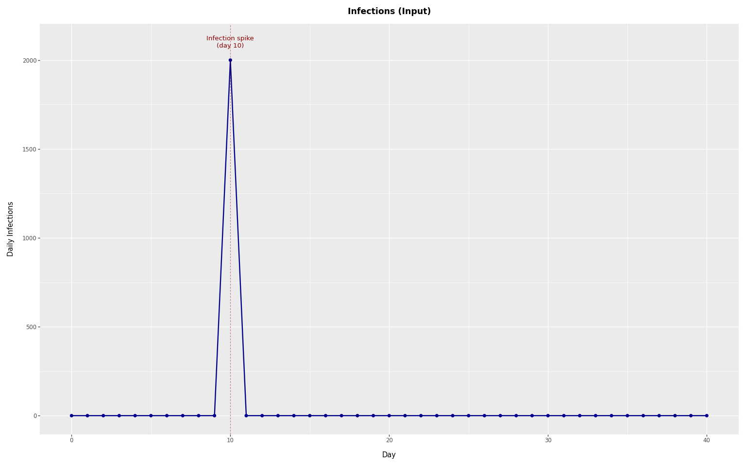
Simulating from observations from a single-day infection spike
To see how infections spread into concentrations via shedding kinetics, we simulate from a single-day spike:
Code
n_days = 50
day_one = first_valid_observation_day(ww_process)

# Create infections with a spike (shape: n_days x n_subpops)
infection_spike_day = day_one + 10
infections = jnp.zeros((n_days, 1))  # 1 subpopulation
infections = infections.at[infection_spike_day, 0].set(2000.0)

# For plotting
rel_spike_day = infection_spike_day - day_one
n_plot_days = n_days - day_one

# Observation times and indices
observation_days = jnp.arange(day_one, 40, dtype=jnp.int32)
n_obs = len(observation_days)

with numpyro.handlers.seed(rng_seed=42):
    ww_obs = ww_process.sample(
        infections=infections,
        subpop_indices=jnp.zeros(n_obs, dtype=jnp.int32),
        sensor_indices=jnp.zeros(n_obs, dtype=jnp.int32),
        times=observation_days,
        obs=None,
        n_sensors=1,
    )
We plot the resulting observations starting from the first valid observation day.
Code
infections_df = pd.DataFrame(
    {
        "day": np.arange(n_plot_days),
        "infections": np.array(infections[day_one:, 0]),
    }
)

max_infection_count = float(jnp.max(infections[day_one:]))

plot_infections = (
    p9.ggplot(infections_df, p9.aes(x="day", y="infections"))
    + p9.geom_line(color="darkblue", size=1)
    + p9.geom_point(color="darkblue", size=2)
    + p9.geom_vline(
        xintercept=rel_spike_day,
        color="darkred",
        linetype="dashed",
        alpha=0.5,
    )
    + p9.labs(x="Day", y="Daily Infections", title="Infections (Input)")
    + theme_tutorial
    + p9.annotate(
        "text",
        x=rel_spike_day,
        y=max_infection_count * 1.05,
        label=f"Infection spike\n(day {rel_spike_day})",
        color="darkred",
        size=10,
        ha="center",
    )
)
plot_infections
Observation noise
Sampling multiple times from the same infections shows the range of possible observations:
Code
n_samples = 50
ww_samples_list = []

for seed in range(n_samples):
    with numpyro.handlers.seed(rng_seed=seed):
        ww_result = ww_process.sample(
            infections=infections,
            subpop_indices=jnp.zeros(n_obs, dtype=jnp.int32),
            sensor_indices=jnp.zeros(n_obs, dtype=jnp.int32),
            times=observation_days,
            obs=None,
            n_sensors=1,
        )
    for day_idx, conc in zip(observation_days, ww_result.observed):
        ww_samples_list.append(
            {
                "day": int(day_idx) - day_one,
                "log_concentration": float(conc),
                "sample": seed,
            }
        )

ww_samples_df = pd.DataFrame(ww_samples_list)
Code
# Compute mean across samples for each day
mean_by_day = ww_samples_df.groupby("day")["log_concentration"].mean().reset_index()
mean_by_day["sample"] = -1

# Relative peak day for plotting (using mode, not mean, since distribution is skewed)
peak_day = rel_spike_day + mode_shedding_day

# Separate one sample to highlight
highlight_sample = 0
other_samples_df = ww_samples_df[ww_samples_df["sample"] != highlight_sample]
highlight_df = ww_samples_df[ww_samples_df["sample"] == highlight_sample]

# For annotation positioning
max_conc = ww_samples_df["log_concentration"].max()

(
    p9.ggplot()
    + p9.geom_line(
        p9.aes(x="day", y="log_concentration", group="sample"),
        data=other_samples_df,
        color="orange",
        alpha=0.15,
        size=0.5,
    )
    + p9.geom_line(
        p9.aes(x="day", y="log_concentration"),
        data=highlight_df,
        color="steelblue",
        size=1,
    )
    + p9.geom_line(
        p9.aes(x="day", y="log_concentration"),
        data=mean_by_day,
        color="darkred",
        size=1.2,
    )
    + p9.geom_vline(
        xintercept=rel_spike_day,
        color="darkblue",
        linetype="dashed",
        alpha=0.5,
    )
    + p9.geom_vline(
        xintercept=peak_day,
        color="darkred",
        linetype="dotted",
        alpha=0.7,
    )
    + p9.annotate(
        "text",
        x=rel_spike_day,
        y=max_conc * 1.05,
        label=f"Infection spike\n(day {rel_spike_day})",
        color="darkblue",
        size=9,
        ha="center",
    )
    + p9.annotate(
        "text",
        x=peak_day,
        y=max_conc * 0.98,
        label=f"Expected peak\n(day {peak_day})",
        color="darkred",
        size=9,
        ha="center",
    )
    + p9.labs(
        x="Day",
        y="Log Viral Concentration",
        title=f"Observation Noise: {n_samples} Samples from Same Infections",
        subtitle="Blue: one realization | Orange: other samples | Dark red: sample mean",
    )
    + theme_tutorial
)
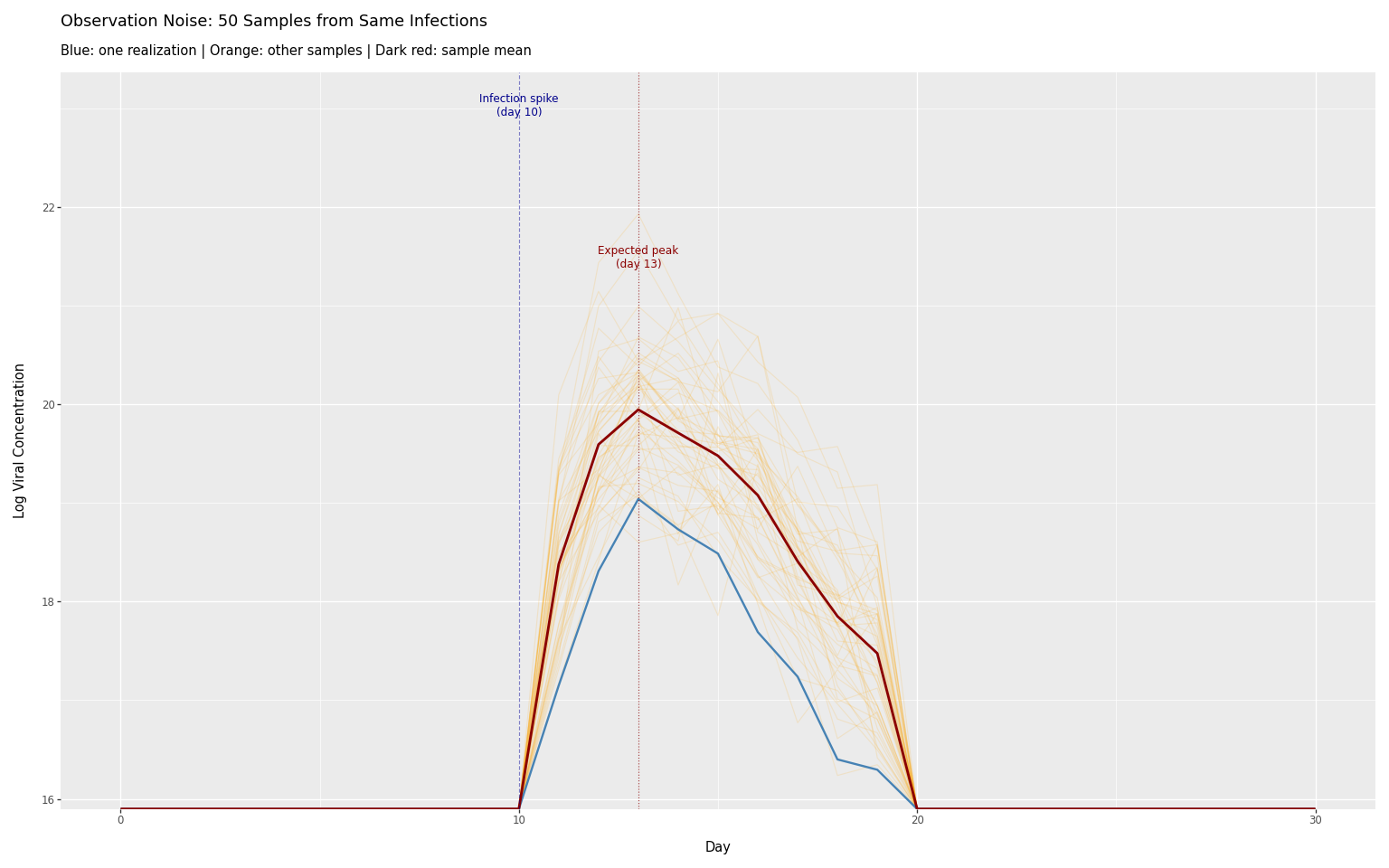
Sensor-level variability
The previous plot showed variability from repeatedly sampling the entire observation process (resampling sensor parameters and noise each time). In practice, we have multiple physical sensors, each with fixed but unknown characteristics.
This plot shows four sensors observing the same infection spike. Each sensor has:
- A sensor mode (systematic bias): shifts all observations up or down
- A sensor SD (measurement precision): determines noise level around predictions
These parameters are sampled once per sensor, then held fixed across all observations from that sensor.
Code
num_sensors = 4

# Use the same observation times and infections as the sampled-concentrations plot
sensor_obs_times = jnp.tile(observation_days, num_sensors)
sensor_ids = jnp.repeat(jnp.arange(num_sensors, dtype=jnp.int32), len(observation_days))
subpop_ids = jnp.zeros(num_sensors * len(observation_days), dtype=jnp.int32)

with numpyro.handlers.seed(rng_seed=42):
    ww_multi_sensor = ww_process.sample(
        infections=infections,  # Same spike as before
        subpop_indices=subpop_ids,
        sensor_indices=sensor_ids,
        times=sensor_obs_times,
        obs=None,
        n_sensors=num_sensors,
    )

# Create DataFrame for plotting (using relative days)
multi_sensor_df = pd.DataFrame(
    {
        "day": np.array(sensor_obs_times) - day_one,
        "log_concentration": np.array(ww_multi_sensor.observed),
        "sensor": [f"Sensor {i}" for i in np.array(sensor_ids)],
    }
)
Code
(
    p9.ggplot(multi_sensor_df, p9.aes(x="day", y="log_concentration", color="sensor"))
    + p9.geom_line(size=1)
    + p9.geom_point(size=2)
    + p9.labs(
        x="Day",
        y="Log Viral Concentration",
        title="Four Sensors Observing the Same Infection Spike",
        color="Sensor",
    )
    + theme_tutorial
)
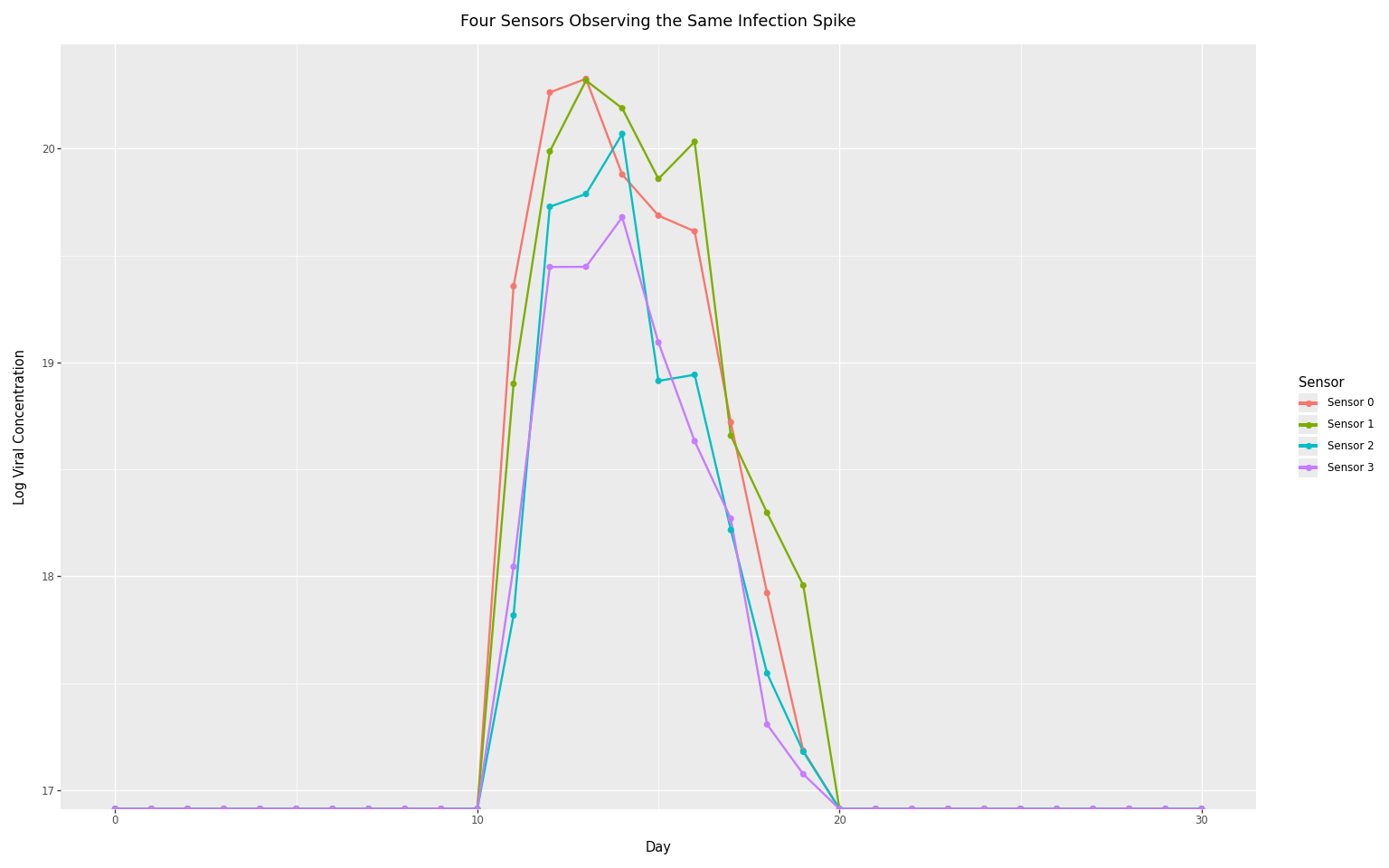
Compare this to the previous plot: here, each colored line represents a distinct physical sensor with its own systematic bias. The vertical spread between sensors reflects differences in sensor modes, while the noise within each line reflects each sensor’s measurement precision. During inference, these sensor-specific effects are learned from data.
Multiple subpopulations
In regional surveillance, each wastewater treatment plant serves a
distinct catchment area (subpopulation) with its own infection
dynamics. The subpop_indices array maps each observation to the
appropriate infection trajectory.
This example shows two subpopulations with different epidemic curves:
- Subpopulation 0: Slow decay (e.g., large urban area with sustained transmission)
- Subpopulation 1: Fast decay (e.g., smaller community with rapid burnout)
Each subpopulation is observed by its own sensor. The observed concentrations reflect both the underlying infection differences AND the sensor-specific measurement characteristics.
Code
# Two subpopulations with different infection patterns
n_days_mp = 40
infections_subpop1 = 1000.0 * jnp.exp(-jnp.arange(n_days_mp) / 20.0)  # Slow decay
infections_subpop2 = 2000.0 * jnp.exp(-jnp.arange(n_days_mp) / 10.0)  # Fast decay
infections_multi = jnp.stack([infections_subpop1, infections_subpop2], axis=1)

# Two sensors, each observing a different subpopulation
obs_days_mp = jnp.tile(jnp.arange(10, 30, 2, dtype=jnp.int32), 2)
subpop_ids_mp = jnp.array([0] * 10 + [1] * 10, dtype=jnp.int32)
sensor_ids_mp = jnp.array([0] * 10 + [1] * 10, dtype=jnp.int32)

with numpyro.handlers.seed(rng_seed=42):
    ww_multi_subpop = ww_process.sample(
        infections=infections_multi,
        subpop_indices=subpop_ids_mp,
        sensor_indices=sensor_ids_mp,
        times=obs_days_mp,
        obs=None,
        n_sensors=2,
    )

# Create DataFrame for plotting
multi_subpop_df = pd.DataFrame(
    {
        "day": np.array(obs_days_mp),
        "log_concentration": np.array(ww_multi_subpop.observed),
        "subpopulation": [f"Subpop {i}" for i in np.array(subpop_ids_mp)],
    }
)
Code
(
    p9.ggplot(
        multi_subpop_df,
        p9.aes(x="day", y="log_concentration", color="subpopulation"),
    )
    + p9.geom_line(size=1)
    + p9.geom_point(size=2)
    + p9.labs(
        x="Day",
        y="Log Viral Concentration",
        title="Two Subpopulations with Different Infection Dynamics",
        color="Subpopulation",
    )
    + theme_tutorial
)
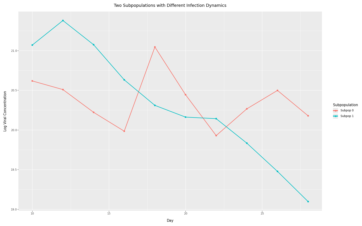
The diverging trajectories reflect the different underlying infection curves. Subpopulation 1 starts higher but decays faster, while Subpopulation 0 maintains more sustained levels. In a full model, you would jointly infer the infection trajectories for each subpopulation while accounting for sensor-specific biases.
Summary
The MeasurementObservation class provides:
- A consistent interface for continuous observation processes
- Hierarchical noise models that capture sensor-level variability
- Flexible indexing for irregular, multi-sensor, multi-subpopulation data
- Convolution utilities with proper timeline alignment
To use it for your domain:
- Subclass
MeasurementObservation - Implement
_predicted_obs()with your signal transformation - Configure appropriate priors for sensor-level effects
- Use the indexing system to map observations to their context