PyRenew’s RandomVariable abstract base class

Design principle: all quantities are RandomVariables

In a Bayesian model, all quantities — data, parameters, hyperparameters, derived computations — are random variables living in a single joint probability model (Gelman et al., BDA3 §1.3). The only distinction is whether a given quantity is known (observed, conditioned on) or unknown (to be inferred). A fixed constant is just a degenerate random variable; an estimated rate is a draw from a prior. Both participate in the same joint distribution.

PyRenew embodies this through its RandomVariable abstract base class. All model components implement the same sample() interface, so you can swap a fixed quantity for an estimated one — or vice versa — without changing any surrounding model code.

import jax.numpy as jnp
import numpy as np
import numpyro
import numpyro.distributions as dist
import pandas as pd
import plotnine as p9
import warnings
from plotnine.exceptions import PlotnineWarning

warnings.filterwarnings("ignore", category=PlotnineWarning)

from pyrenew.metaclass import RandomVariable
from pyrenew.deterministic import DeterministicVariable, DeterministicPMF
from pyrenew.randomvariable import (
    DistributionalVariable,
    StaticDistributionalVariable,
    DynamicDistributionalVariable,
    TransformedVariable,
)
from pyrenew.observation import Counts, NegativeBinomialNoise
import pyrenew.transformation as transformation
from pyrenew import datasets

Concrete implementations

PyRenew provides four RandomVariable implementations that cover most modeling needs.

DeterministicVariable

A degenerate random variable that returns a fixed value. Its sample() method simply returns the stored value, unchanged.

ihr_fixed = DeterministicVariable("ihr", 0.01)

with numpyro.handlers.seed(rng_seed=0):
    value = ihr_fixed()
    print(f"IHR (fixed): {value}")

IHR (fixed): 0.01

DeterministicPMF specializes this for probability mass functions, validating at construction time that the values sum to 1:

delay_pmf = DeterministicPMF(
    "delay",
    jnp.array([0.0, 0.1, 0.3, 0.3, 0.2, 0.1]),
)

with numpyro.handlers.seed(rng_seed=0):
    pmf = delay_pmf()
    print(f"Delay PMF: {np.round(pmf, 2)}, sum: {pmf.sum():.1f}")

Delay PMF: [0.         0.09999999 0.29999998 0.29999998 0.19999999 0.09999999], sum: 1.0

DistributionalVariable

A random variable that draws from a numpyro distribution via numpyro.sample(). The DistributionalVariable factory function dispatches to one of two classes depending on whether the distribution is known at construction time or built at sample time.

StaticDistributionalVariable: the distribution is fully specified at construction time.

# IHR with a Beta(2, 198) prior: mean ~1%, moderate uncertainty
ihr_estimated = DistributionalVariable("ihr", dist.Beta(2, 198))
print(f"Type: {type(ihr_estimated).__name__}")

with numpyro.handlers.seed(rng_seed=0):
    print(f"IHR (sampled): {ihr_estimated():.4f}")

Type: StaticDistributionalVariable
IHR (sampled): 0.0221

DynamicDistributionalVariable: the distribution is constructed at sample time from a callable. This is useful when distribution parameters depend on other sampled quantities.

# A Normal whose location is determined at sample time
dynamic_rv = DistributionalVariable(
    "dynamic_normal",
    lambda loc: dist.Normal(loc, 0.1),
)
print(f"Type: {type(dynamic_rv).__name__}")

with numpyro.handlers.seed(rng_seed=0):
    print(f"Sample (loc=2.0): {dynamic_rv.sample(2.0):.3f}")
    print(f"Sample (loc=5.0): {dynamic_rv.sample(5.0):.3f}")

Type: DynamicDistributionalVariable
Sample (loc=2.0): 1.756
Sample (loc=5.0): 4.874

TransformedVariable

Wraps another RandomVariable and applies a deterministic transformation to its output. This is useful for reparameterizations and derived quantities.

# Day-of-week effect: Dirichlet draw scaled by 7
# so effects are multiplicative and preserve weekly totals
dow_effect = TransformedVariable(
    name="dow_effect",
    base_rv=DistributionalVariable(
        name="dow_raw",
        distribution=dist.Dirichlet(jnp.ones(7)),
    ),
    transforms=transformation.AffineTransform(loc=0, scale=7),
)

with numpyro.handlers.seed(rng_seed=0):
    effect = dow_effect()
    print(f"Day-of-week multipliers: {np.round(effect, 3)}")
    print(f"Sum: {effect.sum():.1f}")

Day-of-week multipliers: [1.789      0.013      0.07       0.21400002 2.7020001  0.508
 1.7040001 ]
Sum: 7.0

Interchangeability

Because all implementations share the sample() interface, you can swap them freely. For example, the Counts observation process accepts any RandomVariable as its ascertainment_rate_rv. The model code is identical whether the rate is fixed or estimated:

hosp_delay_pmf = jnp.array(
    datasets.load_infection_admission_interval()["probability_mass"].to_numpy()
)

# Fixed ascertainment rate
hosp_fixed = Counts(
    name="hospital",
    ascertainment_rate_rv=DeterministicVariable("ihr", 0.01),
    delay_distribution_rv=DeterministicPMF("delay", hosp_delay_pmf),
    noise=NegativeBinomialNoise(DeterministicVariable("conc", 10.0)),
)

# Estimated ascertainment rate --- same model structure, different RV
hosp_estimated = Counts(
    name="hospital",
    ascertainment_rate_rv=DistributionalVariable("ihr", dist.Beta(2, 198)),
    delay_distribution_rv=DeterministicPMF("delay", hosp_delay_pmf),
    noise=NegativeBinomialNoise(DeterministicVariable("conc", 10.0)),
)

The RandomVariable public API

The RandomVariable metaclass (defined in pyrenew.metaclass) requires subclasses to implement:

Method	Signature	Purpose
`sample`	`sample(**kwargs) -> tuple`	Core computation: return a value, draw from a distribution, or perform a calculation
`validate`	`validate(**kwargs) -> None`	Check that parameters are well-formed; raise an error if not

The metaclass also provides:

Method	Behavior
`__call__(**kwargs)`	Alias for `sample(**kwargs)`, so `my_rv()` is equivalent to `my_rv.sample()`

The **kwargs pattern is central to composability: a RandomVariable accepts whatever arguments its sample() method needs, and passes through any additional keyword arguments to internal calls.

Writing a custom RandomVariable

The built-in classes handle most cases, but sometimes you need a component with custom logic—for instance, one that makes multiple numpyro.sample() calls, performs domain-specific validation, or records derived quantities via numpyro.deterministic().

Example: ascertainment with day-of-week effects

Hospital admissions data typically shows day-of-week reporting patterns: fewer admissions are reported on weekends, more on weekdays. We can model this as a multiplicative adjustment to a baseline ascertainment rate.

The predicted hospital admissions on day \(t\) are:

\[\lambda_t = \alpha \cdot w_{t \bmod 7} \cdot \sum_{d=0}^{D} I_{t-d} \cdot p_d\]

where \(\alpha\) is the baseline ascertainment rate, \(w_j\) for \(j = 0, \ldots, 6\) are day-of-week multipliers (positive, summing to 7 so that the weekly total is preserved), and the summation is the delay convolution.

We define a custom RandomVariable that bundles the ascertainment rate and day-of-week effect into a single component, returning a daily rate vector.

from jax.typing import ArrayLike


class AscertainmentWithDayOfWeek(RandomVariable):
    """
    Ascertainment rate modulated by day-of-week reporting effects.

    Combines a scalar ascertainment rate with a 7-element
    day-of-week multiplier to produce a daily rate vector.
    """

    def __init__(
        self,
        name: str,
        baseline_rate_rv: RandomVariable,
        dow_concentration: ArrayLike,
        first_day_offset: int = 0,
    ) -> None:
        """
        Parameters
        ----------
        name
            Name prefix for numpyro sample sites.
        baseline_rate_rv
            RandomVariable for the baseline ascertainment rate.
        dow_concentration
            Dirichlet concentration parameters, shape (7,).
            Larger values produce less day-to-day variation.
        first_day_offset
            Day of the week for the first day of the timeseries
            (0 = Monday, 6 = Sunday).
        """
        self.validate(dow_concentration, first_day_offset)
        super().__init__(name=name)
        self.baseline_rate_rv = baseline_rate_rv
        self.dow_concentration = jnp.asarray(dow_concentration)
        self.first_day_offset = first_day_offset

    @staticmethod
    def validate(dow_concentration, first_day_offset) -> None:
        """Check that parameters are well-formed."""
        dow_concentration = jnp.asarray(dow_concentration)
        if dow_concentration.shape != (7,):
            raise ValueError(
                f"dow_concentration must have shape (7,), "
                f"got {dow_concentration.shape}"
            )
        if jnp.any(dow_concentration <= 0):
            raise ValueError("dow_concentration values must be positive")
        if not (0 <= first_day_offset <= 6):
            raise ValueError(
                f"first_day_offset must be 0-6, got {first_day_offset}"
            )

    def sample(self, n_days: int, **kwargs) -> tuple:
        """
        Sample a daily ascertainment rate vector.

        Parameters
        ----------
        n_days
            Number of days in the timeseries.

        Returns
        -------
        tuple
            Containing a single array of daily ascertainment rates,
            shape (n_days,).
        """
        # Sample baseline rate (delegates to another RandomVariable)
        baseline = self.baseline_rate_rv()
        numpyro.deterministic(f"{self.name}_baseline_rate", baseline)

        # Sample day-of-week effects from Dirichlet, scale to sum to 7
        dow_raw = numpyro.sample(
            f"{self.name}_dow_raw",
            dist.Dirichlet(self.dow_concentration),
        )
        dow_effect = dow_raw * 7.0
        numpyro.deterministic(f"{self.name}_dow_effect", dow_effect)

        # Tile the 7-element vector across the timeseries
        full_cycle = jnp.tile(dow_effect, (n_days // 7) + 1)
        daily_dow = full_cycle[
            self.first_day_offset : self.first_day_offset + n_days
        ]

        # Combine: daily rate = baseline * day-of-week multiplier
        daily_rate = baseline * daily_dow

        return (daily_rate,)

This class bundles three things that belong together:

Two sample statements: one for the baseline rate (delegated to baseline_rate_rv) and one for the Dirichlet day-of-week effects
Derived computation: scaling, tiling, offsetting, and combining into a daily vector
Validation: checking that concentration has shape (7,) and the offset is valid

Sampling from the custom RV

ascertainment_rv = AscertainmentWithDayOfWeek(
    name="hosp",
    baseline_rate_rv=DistributionalVariable("ihr", dist.Beta(2, 198)),
    dow_concentration=jnp.array([5, 5, 5, 5, 5, 2, 2]),  # lower on weekends
    first_day_offset=0,  # timeseries starts on Monday
)

n_days = 28

with numpyro.handlers.seed(rng_seed=42):
    (daily_rates,) = ascertainment_rv(n_days=n_days)

day_labels = ["Mon", "Tue", "Wed", "Thu", "Fri", "Sat", "Sun"]

rates_df = pd.DataFrame(
    {
        "day": np.arange(n_days),
        "rate": np.array(daily_rates),
        "dow": [day_labels[i % 7] for i in range(n_days)],
        "day_type": [
            "Weekend" if i % 7 >= 5 else "Weekday" for i in range(n_days)
        ],
    }
)

(
    p9.ggplot(rates_df, p9.aes(x="day", y="rate", fill="day_type"))
    + p9.geom_col(alpha=0.7, color="black", size=0.3)
    + p9.scale_fill_manual(
        values={"Weekday": "lightblue", "Weekend": "orange"}
    )
    + p9.labs(
        x="Day",
        y="Daily Ascertainment Rate",
        title="Ascertainment Rate with Day-of-Week Effects",
        fill="",
    )
    + p9.theme_grey()
    + p9.theme(plot_title=p9.element_text(size=14, weight="bold"))
)

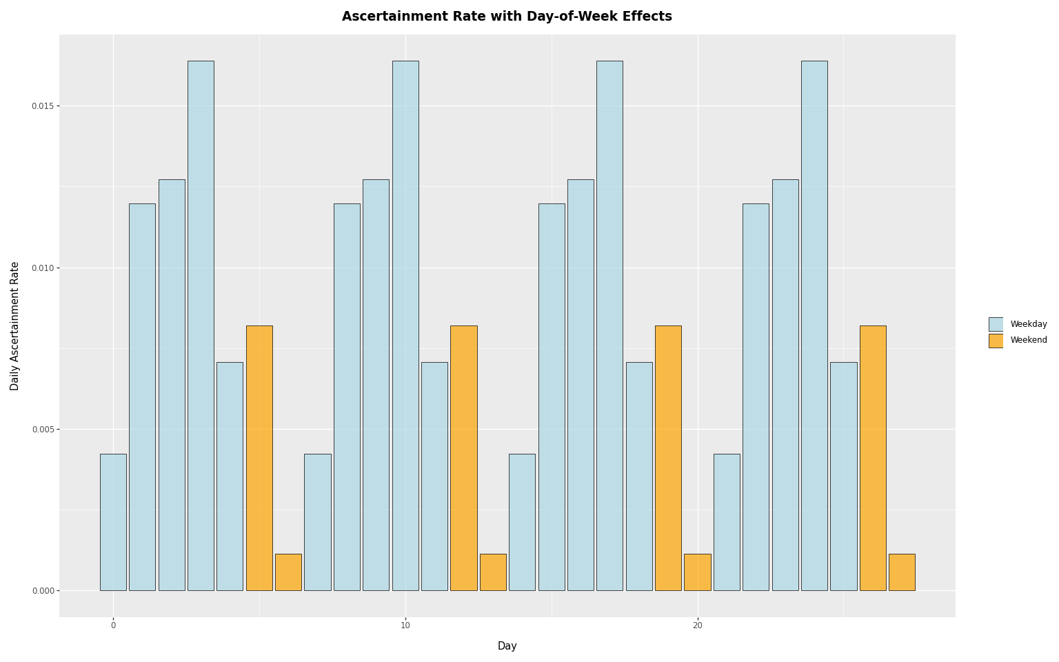
The weekly pattern is clear: weekday rates are higher than weekend rates, reflecting reduced reporting on weekends.

Applying to a simulated observation process

We now use the AscertainmentWithDayOfWeek instance defined above to generate day-of-week multipliers within a realistic observation pipeline, showing how a custom RandomVariable integrates into a data-generating process.

In a hospital surveillance system, the observation pipeline is:

Infections occur over time (the latent process).
Delay: each infection leads to a hospital admission after some delay, modeled as a convolution with a delay PMF.
Reporting: the admission is reported with day-of-week effects — fewer reports on weekends, more on weekdays.
Noise: observed counts include measurement noise.

The day-of-week effect is a reporting artifact, so it is applied after the delay convolution. We walk through each step explicitly to make the pipeline clear.

# Epidemic curve: exponential growth then decay
n_days = 60
infections = 10000.0 * jnp.exp(-((jnp.arange(n_days) - 25.0) ** 2) / 200.0)

We convolve infections with the delay PMF and apply a baseline ascertainment rate to get the expected admissions before noise:

baseline_rate = 0.01
expected_admissions = jnp.convolve(
    baseline_rate * infections,
    hosp_delay_pmf,
    mode="full",
)[:n_days]

Now we simulate observed admissions with and without day-of-week effects. Without effects, we add noise directly to the smooth expected curve. With effects, we first call our custom ascertainment_rv to get a day-of-week multiplier, apply it to the expected admissions (post-convolution, at the reporting stage), then add noise.

n_samples = 20
concentration = 50.0

results = []
for seed in range(n_samples):
    with numpyro.handlers.seed(rng_seed=seed):
        # Without day-of-week: noise on the smooth expected curve
        obs_no_dow = numpyro.sample(
            "obs_no_dow",
            dist.NegativeBinomial2(expected_admissions, concentration),
        )

    with numpyro.handlers.seed(rng_seed=seed + 1000):
        # Sample day-of-week multiplier from the custom RV
        (daily_rates,) = ascertainment_rv(n_days=n_days)
        dow_multiplier = daily_rates / daily_rates.mean()

        # Apply day-of-week *after* the delay convolution
        obs_with_dow = numpyro.sample(
            "obs_with_dow",
            dist.NegativeBinomial2(
                expected_admissions * dow_multiplier, concentration
            ),
        )

    for i in range(n_days):
        results.append(
            {
                "day": i,
                "admissions": float(obs_no_dow[i]),
                "type": "No day-of-week effect",
                "sample": seed,
            }
        )
        results.append(
            {
                "day": i,
                "admissions": float(obs_with_dow[i]),
                "type": "With day-of-week effect",
                "sample": seed,
            }
        )

results_df = pd.DataFrame(results)

(
    p9.ggplot(
        results_df,
        p9.aes(x="day", y="admissions", group="sample"),
    )
    + p9.geom_line(alpha=0.3, size=0.5, color="steelblue")
    + p9.facet_wrap("~ type", ncol=2)
    + p9.labs(
        x="Day",
        y="Hospital Admissions",
        title="Simulated Hospital Admissions",
    )
    + p9.theme_grey()
    + p9.theme(plot_title=p9.element_text(size=14, weight="bold"))
)

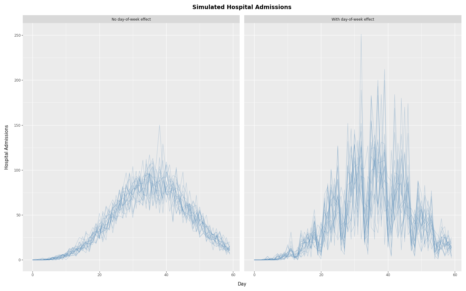
The left panel shows smooth variation from noise alone. The right panel shows the additional weekly oscillation introduced by day-of-week reporting effects — the sawtooth pattern of weekend dips and weekday peaks that is characteristic of real hospital admissions data.

Summary

Choosing a RandomVariable implementation

Need	Use
Fixed known value	`DeterministicVariable`
Fixed known PMF	`DeterministicPMF`
Sample from a fixed distribution	`DistributionalVariable` (static)
Sample from a distribution parameterized at sample time	`DistributionalVariable` (dynamic, pass a callable)
Deterministic transformation of another RV	`TransformedVariable`
Multiple sample statements, custom validation, or derived computation	Custom `RandomVariable` subclass

Writing a custom RandomVariable

Subclass RandomVariable from pyrenew.metaclass
Implement validate() as a @staticmethod; call it in __init__
Implement sample(**kwargs) returning a tuple
Use numpyro.sample() for quantities to be estimated
Use numpyro.deterministic() to record derived quantities in the trace
Accept **kwargs in sample() for composability