Building Multi-Signal Renewal Models

Code

import numpyro

# to run samplers in parallel you must run `set_host_device_count` before importing jax
numpyro.set_host_device_count(4)
numpyro.enable_x64()

Code

import arviz as az
import jax
import jax.numpy as jnp
import jax.random as random
import numpy as np
import numpyro.distributions as dist
import plotnine as p9
import pandas as pd
import time
import warnings

warnings.filterwarnings("ignore")


def make_rng_key():
    """Generate a time-based random seed."""
    seed = int(time.time() * 1000) % (2**32)
    return random.PRNGKey(seed)

/home/runner/work/PyRenew/PyRenew/.venv/lib/python3.14/site-packages/arviz/__init__.py:50: FutureWarning: 
ArviZ is undergoing a major refactor to improve flexibility and extensibility while maintaining a user-friendly interface.
Some upcoming changes may be backward incompatible.
For details and migration guidance, visit: https://python.arviz.org/en/latest/user_guide/migration_guide.html
  warn(

Code

from jax.typing import ArrayLike

from pyrenew import datasets
from pyrenew.deterministic import (
    DeterministicPMF,
    DeterministicVariable,
)
from pyrenew.metaclass import RandomVariable
from pyrenew.randomvariable import DistributionalVariable

from pyrenew.latent import (
    HierarchicalInfections,
    AR1,
    RandomWalk,
    GammaGroupSdPrior,
    HierarchicalNormalPrior,
)
from pyrenew.model import PyrenewBuilder

from pyrenew.observation import (
    Counts,
    HierarchicalNormalNoise,
    Measurements,
    MeasurementNoise,
    NegativeBinomialNoise,
)

Overview

Renewal models in PyRenew combine two types of components:

Latent infection process: Generates unobserved infections via the renewal equation, driven by a time-varying reproduction number \(\mathcal{R}(t)\)
Observation processes: Transform latent infections into observable signals (hospital admissions, wastewater concentrations, etc.) by applying delays, ascertainment, and noise

A multi-signal model combines multiple observation processes—each representing a different data stream, e.g., hospital admissions, wastewater concentrations, which stem from the same underlying latent infection process. By jointly modeling these signals, we can improve estimation and prediction of the time-varying reproduction number \(\mathcal{R}(t)\). Such a model must:

Generate a single coherent infection trajectory (or set of trajectories for subpopulations)
Route those infections to each observation process appropriately
Handle the initialization period required by delay distributions

The PyrenewBuilder class handles this plumbing. You specify:

A latent process (e.g., HierarchicalInfections) that defines how infections evolve
One or more observation processes (e.g., Counts, Measurements) that define how infections become data

The builder computes initialization requirements, wires components together, and produces a model ready for inference.

Before diving into multi-signal models, you may want to review these foundational tutorials:

Hierarchical Latent Infections: Understanding temporal process choices for \(\mathcal{R}(t)\)
Observation Processes: Counts: Modeling count data (admissions, deaths)
Observation Processes: Measurements: Modeling continuous data (wastewater)

This tutorial shows how to combine these components into a complete multi-signal model.

What This Tutorial Covers

This tutorial demonstrates building a multi-signal renewal model using:

HierarchicalInfections — subpopulations share a jurisdiction-level baseline \(\mathcal{R}(t)\) with subpopulation-specific deviations
Counts — hospital admissions (jurisdiction-level)
A custom Wastewater class — viral concentrations (subpopulation-level)

Model Structure

In this tutorial, we build a model that jointly fits two data streams to a shared latent infection process:

Hospital admissions — jurisdiction-level counts that reflect total infections across all subpopulations, delayed and underascertained
Wastewater concentrations — site-level measurements from a subset of subpopulations (catchment areas), reflecting viral shedding and dilution

The diagram below shows how data flows through the model. The latent process generates infection trajectories for all subpopulations. Each observation process receives the infections it needs — aggregated totals or per-subpopulation arrays — and transforms them into predicted observations via delays, ascertainment, shedding kinetics, and noise.

flowchart TB

    subgraph Latent["Latent Infection Process"]
        L["Renewal equation<br/>(HierarchicalInfections)"]
    end

    subgraph Infections["Infection Trajectories"]
        J["Jurisdiction total<br/>(summed across subpopulations)"]
        S["Per-subpopulation infections<br/>(all subpopulations)"]
    end

    subgraph Obs["Observation Processes"]
        C["Hospital admissions<br/>(Counts)"]
        W["Wastewater concentrations<br/>(Measurements)"]
    end

    subgraph Data["Observed Data"]
        HA["Reported admissions"]
        WW["Measured viral concentrations"]
    end

    L --> S
    S -->|"weighted sum"| J
    J --> C
    S -->|"select monitored subpopulations"| W
    C -->|"delay + ascertainment + noise"| HA
    W -->|"shedding + dilution + noise"| WW

Infection Resolution

Different observation processes observe different levels of the model hierarchy. Each observation process declares an infection resolution that determines what infection data it receives:

Resolution	Receives	Example signals
`"aggregate"`	Aggregated infections (sum across all subpopulations), shape `(T,)`	Hospital admissions, case counts
`"subpop"`	Infection matrix for all subpopulations, shape `(T, n_subpops)`	Wastewater, site-specific surveillance

The PyrenewBuilder routes latent infections to observation processes based on each process’s declared resolution.

For subpopulation-level observations, the observation process selects which subpopulations it observes using subpop_indices provided at sample/fit time. This allows flexible observation patterns—for example, wastewater samples might only cover 5 of 6 subpopulations (catchment areas), while the 6th represents areas without wastewater monitoring.

With this structure in mind, we’ll now define each component following the generative direction: first the latent infection process, then the observation processes.

Latent Infection Process

Latent infection processes implement the renewal equation to generate infection trajectories. All latent processes share common components:

Generation interval: PMF for secondary infection timing
Initial infections (I0): Starting condition for the renewal process
Temporal dynamics: How \(\mathcal{R}(t)\) evolves over time

Generation Interval

The generation interval PMF specifies the probability that a secondary infection occurs \(d\) days after the primary infection.

Code

covid_gen_int = [0.16, 0.32, 0.25, 0.14, 0.07, 0.04, 0.02]
gen_int_pmf = jnp.array(covid_gen_int)
gen_int_rv = DeterministicPMF("gen_int", gen_int_pmf)

# Mean generation time
days = np.arange(len(gen_int_pmf))
print(f"Generation interval length: {len(gen_int_pmf)} days")

Generation interval length: 7 days

I0: Initial Infections

The initial infections RV I0_rv specifies the proportion of the population infected at the first observation time. This must be a value in the interval (0, 1]. We use a Beta prior centered near a small value:

Code

I0_rv = DistributionalVariable("I0", dist.Beta(1, 100))

Initial Log Rt

We place a prior on the initial log(Rt), centered at 0.0 (Rt = 1.0) with moderate uncertainty:

Code

initial_log_rt_rv = DistributionalVariable(
    "initial_log_rt", dist.Normal(0.0, 0.5)
)

Temporal Processes for \(\mathcal{R}(t)\)

We configure two temporal processes:

Jurisdiction-level (baseline_rt_process): AR(1) process for the baseline \(\mathcal{R}(t)\)
Subpopulation-level (subpop_rt_deviation_process): RandomWalk for subpopulation deviations

The RandomWalk allows flexible evolution of subpopulation-specific transmission without mean reversion.

Code

# AR1 provides mean-reverting behavior for baseline Rt
baseline_rt_process = AR1(autoreg=0.9, innovation_sd=0.05)

# RandomWalk allows flexible subpopulation deviations
subpop_rt_deviation_process = RandomWalk(innovation_sd=0.025)

Observation Processes

Observation processes transform latent infections into observable signals and define the statistical model linking predictions to data. Each observation process:

Has a unique name that identifies the signal in model outputs
Declares what infection resolution it needs ("aggregate" or "subpop")
Applies signal-specific transformations (ascertainment, delay convolution, shedding kinetics)
Defines the noise model

Signal Naming

Each observation process requires a name parameter—a short, meaningful identifier like "hospital" or "wastewater". This name serves as the single identifier for the signal throughout the model:

Numpyro sites: Prefixes all sample and deterministic sites (e.g., hospital_obs, hospital_predicted)
Data binding: Becomes the keyword argument for passing data to model.run() (e.g., hospital={...})

This unified naming provides several benefits:

Interpretable outputs: When examining MCMC samples or posterior diagnostics, site names like hospital_predicted immediately indicate which signal each quantity refers to
Multiple signals of the same type: You can include multiple count observations (e.g., hospital admissions and deaths) by giving each a distinct name
Clearer debugging: Error messages and trace inspection show meaningful signal names rather than generic identifiers

Hospital Admissions

In this example we use a dataset consisting of hospital admissions for COVID-19 across California for the first 10 months of 2023 (as reported to the CDC).

Code

# Load daily hospital admissions for California
ca_hosp_data = datasets.load_hospital_data_for_state("CA", "2023-11-06.csv")

hosp_admits = ca_hosp_data["daily_admits"]
population_size = ca_hosp_data["population"]
n_hosp_days = ca_hosp_data["n_days"]

print("State: California")
print(f"Population: {population_size:,}")
print(f"Date range: {ca_hosp_data['dates'][0]} to {ca_hosp_data['dates'][-1]}")
print(f"Number of days: {n_hosp_days}")
print(
    f"Admissions range: {int(hosp_admits.min())} to {int(hosp_admits.max())}"
)

State: California
Population: 39,512,223
Date range: 2023-01-01 to 2023-11-06
Number of days: 310
Admissions range: 2 to 2574

The hospital admissions data is aggregated at the jurisdiction level, therefore we specify a Counts observation process.

Code

# Infection-to-hospitalization delay (COVID-19, from literature)
inf_to_hosp_pmf = jnp.array(
    [
        0,
        0.00469,
        0.01452,
        0.02786,
        0.04237,
        0.05581,
        0.06657,
        0.07379,
        0.07729,
        0.07737,
        0.07465,
        0.06988,
        0.06377,
        0.05696,
        0.04996,
        0.04315,
        0.03677,
        0.03097,
        0.02583,
        0.02135,
        0.01751,
        0.01427,
        0.01156,
        0.00931,
        0.00746,
        0.00596,
        0.00474,
        0.00375,
        0.00296,
        0.00233,
        0.00183,
        0.00143,
        0.00107,
        0.00077,
        0.00054,
        0.00036,
        0.00024,
        0.00015,
        0.00009,
        0.00005,
        0.00003,
        0.00002,
        0.00001,
    ]
)
hosp_delay_rv = DeterministicPMF("inf_to_hosp_delay", inf_to_hosp_pmf)

# IHR: ~1% of infections lead to hospitalization
ihr_rv = DeterministicVariable("ihr", 0.01)

# Negative binomial concentration (moderate overdispersion)
hosp_concentration_rv = DeterministicVariable("hosp_concentration", 10.0)

# Create hospital observation process
hosp_obs = Counts(
    name="hospital",
    ascertainment_rate_rv=ihr_rv,
    delay_distribution_rv=hosp_delay_rv,
    noise=NegativeBinomialNoise(hosp_concentration_rv),
)

print("Hospital observation:")
print(f"  Infection resolution: {hosp_obs.infection_resolution()}")
print(f"  Delay PMF length: {len(inf_to_hosp_pmf)} days")

Hospital observation:
  Infection resolution: aggregate
  Delay PMF length: 43 days

Wastewater Concentrations

Wastewater Observation Process

The Measurements base class handles continuous observation processes. Domain-specific implementations subclass it and implement _predicted_obs() to transform infections into predicted values. See observation_processes_measurements.md for a detailed tutorial.

Code

class Wastewater(Measurements):
    """
    Wastewater viral concentration observation process.

    Transforms site-level infections into predicted log-concentrations
    via shedding kinetics convolution and genome/volume scaling.
    """

    def __init__(
        self,
        name: str,
        shedding_kinetics_rv: RandomVariable,
        log10_genome_per_infection_rv: RandomVariable,
        ml_per_person_per_day: float,
        noise: MeasurementNoise,
    ) -> None:
        super().__init__(
            name=name, temporal_pmf_rv=shedding_kinetics_rv, noise=noise
        )
        self.log10_genome_per_infection_rv = log10_genome_per_infection_rv
        self.ml_per_person_per_day = ml_per_person_per_day

    def validate(self) -> None:
        shedding_pmf = self.temporal_pmf_rv()
        self._validate_pmf(shedding_pmf, "shedding_kinetics_rv")
        self.noise.validate()

    def lookback_days(self) -> int:
        return len(self.temporal_pmf_rv()) - 1

    def _predicted_obs(self, infections: ArrayLike) -> ArrayLike:
        shedding_pmf = self.temporal_pmf_rv()
        log10_genome = self.log10_genome_per_infection_rv()

        def convolve_site(site_infections):
            convolved, _ = self._convolve_with_alignment(
                site_infections, shedding_pmf, p_observed=1.0
            )
            return convolved

        shedding_signal = jax.vmap(convolve_site, in_axes=1, out_axes=1)(
            infections
        )
        genome_copies = 10**log10_genome
        concentration = (
            shedding_signal * genome_copies / self.ml_per_person_per_day
        )
        return jnp.log(concentration)

Wastewater Data

For the wastewater data, we use a simulated dataset for California with realistic noise patterns that covers the same time period.

Code

# Load wastewater data for California
ca_ww_data = datasets.load_wastewater_data_for_state("CA", "fake_nwss.csv")

ww_conc = ca_ww_data["observed_conc"]  # log concentrations
ww_site_ids = ca_ww_data["site_ids"]
ww_time_indices = ca_ww_data["time_indices"]
ww_n_sites = ca_ww_data["n_sites"]
ww_n_obs = ca_ww_data["n_obs"]
ww_wwtp_names = ca_ww_data["wwtp_names"]

print("State: California")
print(f"Number of sites: {ww_n_sites}")
print(f"Number of observations: {ww_n_obs}")
print(f"Date range: {ca_ww_data['dates'][0]} to {ca_ww_data['dates'][-1]}")
print(
    f"Time index range: {int(ww_time_indices.min())} to {int(ww_time_indices.max())}"
)
print("\nSites:")
for i, name in enumerate(ww_wwtp_names[:5]):
    print(f"  {i}: {name}")
if ww_n_sites > 5:
    print(f"  ... and {ww_n_sites - 5} more")

State: California
Number of sites: 5
Number of observations: 1495
Date range: 2023-01-01 to 2023-11-06
Time index range: 0 to 309

Sites:
  0: 1
  1: 2
  2: 3
  3: 4
  4: 5

Wastewater observations are site-level: each measurement is associated with a specific measurement site. The Wastewater observation process uses LogNormalNoise, which takes hierarchical priors for the site-level mode and standard deviation parameters. This enables partial pooling across measurement sites.

Here we specify HierarchicalNormalPrior for the site-level mode and GammaGroupSdPrior for the standard deviation.

Code

# Viral shedding kinetics PMF (days post-infection)
shedding_pmf = jnp.array(
    [
        0.0,
        0.02,
        0.08,
        0.15,
        0.20,
        0.18,
        0.14,
        0.10,
        0.06,
        0.04,
        0.02,
        0.01,
    ]
)
shedding_pmf = shedding_pmf / shedding_pmf.sum()  # normalize
shedding_rv = DeterministicPMF("shedding_kinetics", shedding_pmf)

# Log10 genomes shed per infection
log10_genome_rv = DeterministicVariable("log10_genome_per_inf", 9.0)

# Wastewater volume per person per day (mL)
ml_per_person_per_day = 1000.0

# Hierarchical priors for site-level effects
site_mode_prior = HierarchicalNormalPrior(
    "ww_site_mode", sd_rv=DeterministicVariable("site_mode_sd", 0.5)
)
site_sd_prior = GammaGroupSdPrior(
    "ww_site_sd",
    sd_mean_rv=DeterministicVariable("site_sd_mean", 0.3),
    sd_concentration_rv=DeterministicVariable("site_sd_conc", 4.0),
)

# Create wastewater observation process
ww_obs = Wastewater(
    name="wastewater",
    shedding_kinetics_rv=shedding_rv,
    log10_genome_per_infection_rv=log10_genome_rv,
    ml_per_person_per_day=ml_per_person_per_day,
    noise=HierarchicalNormalNoise(site_mode_prior, site_sd_prior),
)

print("Wastewater observation:")
print(f"  Infection resolution: {ww_obs.infection_resolution()}")
print(f"  Shedding PMF length: {len(shedding_pmf)} days")

Wastewater observation:
  Infection resolution: subpop
  Shedding PMF length: 12 days

Model Building

We instantiate a PyrenewBuilder object which handles the composition of the latent infection process and the observation process.

Code

# Build the multi-signal model
builder = PyrenewBuilder()

The PyrenewBuilder object has 3 key methods:

configure_latent
add_observation
build

Methods configure_latent and add_observation can be called in any order. Method build is called once all processes have been specified in the model.

Configuring the Latent Process

We use configure_latent to specify the model structure: generation interval, initial infections, and temporal dynamics.

Code

print("Latent process configuration:")
print(f"  Generation interval length: {len(gen_int_rv())} days")

builder.configure_latent(
    HierarchicalInfections,
    gen_int_rv=gen_int_rv,
    I0_rv=I0_rv,
    initial_log_rt_rv=initial_log_rt_rv,
    baseline_rt_process=baseline_rt_process,
    subpop_rt_deviation_process=subpop_rt_deviation_process,
)

Latent process configuration:
  Generation interval length: 7 days

<pyrenew.model.pyrenew_builder.pyrenewbuilder 0x7f2fac1bf620="" at="">

Specifying the Observation Processes, Data

Each observation process’s name attribute becomes the keyword used to pass that observation’s data to model.run() (e.g., hospital={...}, wastewater={...}).

Code

builder.add_observation(hosp_obs)  # Uses hosp_obs.name = "hospital"
builder.add_observation(ww_obs)  # Uses ww_obs.name = "wastewater"
model = builder.build()

n_init = model.latent.n_initialization_points
print("Model built successfully")
print(f"  n_initialization_points: {n_init}")
print(f"  Latent process: {type(model.latent).__name__}")
print(f"  Observation processes: {list(model.observations.keys())}")

Model built successfully
  n_initialization_points: 42
  Latent process: HierarchicalInfections
  Observation processes: ['hospital', 'wastewater']

Fitting the Model to Data: `model.run()`

When you call model.run(), you supply two types of information:

Observation data — one data dictionary per registered observation process
Population structure — how the jurisdiction is divided into subpopulations

Shared Time Axis

All observation data uses a shared time axis [0, n_total) where n_total = n_init + n_days. This shared axis aligns observations with the internal infection vectors:

Index 0 corresponds to the first day of the initialization period
Index n_init corresponds to the first day of actual observations
Index n_total - 1 corresponds to the last observation day

The model provides helper methods to align your data with this shared axis:

model.pad_observations(obs) — prepends n_init NaN values to dense observation vectors
model.shift_times(times) — adds n_init to sparse time indices

Observation Data by Signal Type

Each observation process’s name attribute becomes the keyword argument for passing data to model.run():

builder.add_observation(hosp_obs)   # hosp_obs.name="hospital" → hospital={...}
builder.add_observation(ww_obs)     # ww_obs.name="wastewater" → wastewater={...}

Jurisdiction-level signals (dense)

The jurisdiction-level hospital admissions data is specified as a Counts observations process with dense data padded to length n_total:

hospital={
    "obs": model.pad_observations(hosp_counts),  # shape: (n_total,), NaN-padded
}

The pad_observations method prepends n_init NaN values. NaN marks the initialization period where predictions exist but observations do not. You can also use NaN to mark missing data within the observation period.

Subpopulation-level signals (sparse)

The subpopulation-level wastewater data is specified as a Wastewater observations process with sparse indexing on the shared time axis:

wastewater={
    "obs": jnp.array([...]),                      # observed log concentrations (n_obs,)
    "times": model.shift_times(ww_times),         # time indices on shared axis
    "subpop_indices": jnp.array([...]),           # which subpopulation (selects infection column)
    "sensor_indices": jnp.array([...]),           # which WWTP/lab pair (selects noise parameters)
    "n_sensors": int,                             # total number of WWTP/lab pairs
}

The shift_times method adds n_init to convert from natural coordinates (0 = first observation day) to the shared time axis.

Understanding subpop_indices: The latent process generates infections for all subpopulations as a matrix of shape (T, n_subpops). Each observation selects which column (subpopulation) it came from using subpop_indices. This is how observation processes “know” which subpopulations they observe—the user specifies this mapping at sample/run time.

A subpopulation is a portion of the jurisdiction’s population (e.g., a catchment area). A sensor is a measurement source — typically a WWTP/lab pair — that produces observations. Multiple sensors can observe the same subpopulation (e.g., different labs processing samples from the same catchment), so subpop_indices and sensor_indices may differ.

subpop_indices links each observation to the appropriate infection column (0-indexed into the subpopulations)
sensor_indices selects which sensor’s noise parameters (mode and sd) to apply

Example: A jurisdiction has 6 subpopulations (indices 0-5), where 5 have wastewater monitoring and 1 does not. The subpop_fractions array has 6 elements. If subpopulation 2 lacks wastewater monitoring, wastewater observations would have subpop_indices values only in {0, 1, 3, 4, 5}—never 2. The monitored subpopulations need not be contiguous. The latent process still generates infections for all 6 subpopulations; the wastewater observation just doesn’t see subpopulation 2.

Population Structure

Population structure is specified via a single array of fractions for all subpopulations:

model.run(
    ...,
    subpop_fractions=jnp.array([...]),  # one fraction per subpopulation, must sum to 1
)

This specifies 6 subpopulations with their population fractions. The fractions must sum to 1.0. The latent process generates infections for all 6 subpopulations.

Which subpopulations each observation process “sees” is determined by the subpop_indices in the observation data, not by the population structure. For example, if wastewater monitoring covers only 5 of the 6 subpopulations (say, all except subpopulation 2), the wastewater observation data would have subpop_indices values in {0, 1, 3, 4, 5} but never 2. The monitored subpopulations can be any subset of {0, …, n_subpops-1}.

Example `model.run()` Call

model.run(
    num_warmup=500,
    num_samples=500,
    mcmc_args={"num_chains": 4, "progress_bar": False},
    # Model arguments (passed through to sample())
    n_days_post_init=n_days,
    population_size=population_size,
    subpop_fractions=subpop_fractions,
    hospital={"obs": model.pad_observations(hosp_counts)},
    wastewater={
        "obs": ww_conc,
        "times": model.shift_times(ww_times),
        "subpop_indices": ww_subpop_indices,
        "sensor_indices": ww_sensor_indices,
        "n_sensors": n_ww_sensors,
    },
)
samples = model.mcmc.get_samples()

Running the Model

First we declare the population structure. We have 6 subpopulations, where 5 have wastewater monitoring and 1 does not. The subpopulations with wastewater monitoring need not be contiguous indices—they could be any subset of {0, 1, …, n_subpops-1}.

Code

# All 6 subpopulations with their population fractions
subpop_fractions = jnp.array([0.10, 0.14, 0.21, 0.22, 0.07, 0.26])

n_subpops = len(subpop_fractions)

# Which subpopulations have wastewater monitoring?
# These indices will be used in subpop_indices for wastewater observations.
# They can be any subset of {0, 1, ..., n_subpops-1}, not necessarily contiguous.
ww_monitored_subpops = jnp.array(
    [0, 1, 2, 3, 4]
)  # subpop 5 has no wastewater monitoring

print(f"Total subpopulations: {n_subpops}")
print(
    f"Subpopulations with wastewater monitoring: {list(ww_monitored_subpops)}"
)
print(
    f"Wastewater coverage: {float(jnp.sum(subpop_fractions[ww_monitored_subpops])):.0%}"
)
print(f"Total population: {float(jnp.sum(subpop_fractions)):.0%}")

Total subpopulations: 6
Subpopulations with wastewater monitoring: [Array(0, dtype=int64), Array(1, dtype=int64), Array(2, dtype=int64), Array(3, dtype=int64), Array(4, dtype=int64)]
Wastewater coverage: 74%
Total population: 100%

We define a function to prepare observation data using the model’s helper methods to align with the shared time axis.

Code

def prepare_observation_data(
    model, n_days_fit, hosp_admits, ww_data, ww_monitored_subpops
):
    """
    Prepare observation data for fitting.

    Uses model.pad_observations() and model.shift_times() to align data
    with the shared time axis.

    Parameters
    ----------
    model : MultiSignalModel
        The model (provides padding/shifting helpers)
    n_days_fit : int
        Number of days to include in fit
    hosp_admits : array
        Hospital admissions time series
    ww_data : dict
        Wastewater data dictionary
    ww_monitored_subpops : array
        Indices of subpopulations that have wastewater monitoring.
        These are the valid values for subpop_indices in wastewater data.
    """
    # Hospital: dense, NaN-padded to length n_total
    hosp_obs = model.pad_observations(hosp_admits[:n_days_fit])

    # Wastewater: sparse, times shifted to shared axis
    ww_mask = ww_data["time_indices"] < n_days_fit
    ww_times = model.shift_times(ww_data["time_indices"][ww_mask])
    ww_conc = ww_data["observed_conc"][ww_mask]
    ww_sensors = ww_data["site_ids"][ww_mask]

    # Map wastewater sensors to subpopulation indices
    # Each sensor is assigned to one of the monitored subpopulations.
    # In practice, this mapping comes from your data (which WWTP serves which catchment).
    # For this demo, we cycle sensors through the monitored subpopulations.
    n_ww_sensors = ww_data["n_sites"]
    n_monitored = len(ww_monitored_subpops)
    sensor_to_subpop = {
        i: int(ww_monitored_subpops[i % n_monitored])
        for i in range(n_ww_sensors)
    }
    ww_subpop_indices = jnp.array(
        [sensor_to_subpop[int(s)] for s in ww_sensors]
    )

    return {
        "hospital": {
            "obs": hosp_obs,
        },
        "wastewater": {
            "obs": ww_conc,
            "times": ww_times,
            "subpop_indices": ww_subpop_indices,
            "sensor_indices": ww_sensors,
            "n_sensors": n_ww_sensors,
        },
    }

Fit: 90 Days

Putting this altogether, we align the data with the model time and call model.run(). We run 4 sampler chains.

Code

# Clear JAX caches to avoid interference from earlier cells
jax.clear_caches()

n_days_90 = 90
obs_data_90 = prepare_observation_data(
    model, n_days_90, hosp_admits, ca_ww_data, ww_monitored_subpops
)

print(f"Fitting model with {n_days_90} days of data...")
print("  This may take a few minutes...")

start_time = time.time()
model.run(
    num_warmup=500,
    num_samples=500,
    rng_key=make_rng_key(),
    mcmc_args={"num_chains": 4, "progress_bar": False},
    n_days_post_init=n_days_90,
    population_size=population_size,
    subpop_fractions=subpop_fractions,
    **obs_data_90,
)
# JAX uses asynchronous dispatch, so we must block until sampling completes
# to get accurate timing
samples_90 = model.mcmc.get_samples()
jax.block_until_ready(samples_90)
elapsed_90 = time.time() - start_time
print(f"Elapsed time: {elapsed_90:.1f} seconds")

Fitting model with 90 days of data...
  This may take a few minutes...
Elapsed time: 104.0 seconds

Code

lat_inf_90 = samples_90["latent_infections"]
print(f"Posterior samples shape: {lat_inf_90.shape}")
print(f"Mean latent infections: {np.mean(lat_inf_90):,.0f}")

Posterior samples shape: (2000, 132)
Mean latent infections: 303,001

We check that the chains have converged and the number of effective samples.

Code

# ArviZ diagnostics for 90-day fit
def filter_samples_for_arviz(samples, n_init, num_chains=4):
    """Slice time-series samples to exclude initialization period and reshape for chains."""
    num_samples_per_chain = len(list(samples.values())[0]) // num_chains
    filtered = {}
    for k, v in samples.items():
        if v.ndim == 2 and v.shape[1] > n_init:
            # Time-series: slice to post-init period, reshape to (chains, draws, time)
            filtered[k] = v[:, n_init:].reshape(
                num_chains, num_samples_per_chain, -1
            )
        elif v.ndim == 1:
            # Scalar: reshape to (chains, draws)
            filtered[k] = v.reshape(num_chains, num_samples_per_chain)
        else:
            # Multi-dim: reshape to (chains, draws, ...)
            filtered[k] = v.reshape(
                num_chains, num_samples_per_chain, *v.shape[1:]
            )
    return filtered


samples_90_filtered = filter_samples_for_arviz(
    samples_90, n_init, num_chains=2
)
idata_90 = az.from_dict(posterior=samples_90_filtered)
az.summary(idata_90, var_names=["~latent_infections", "~expected"])

arviz - WARNING - Array contains NaN-value.

	mean	sd	hdi_3%	hdi_97%	mcse_mean	mcse_sd	ess_bulk	ess_tail	r_hat
I0	0.061	0.023	0.023	0.105	0.001	0.001	1858.0	1525.0	1.0
hospital_predicted[0]	1581.162	155.473	1300.020	1883.266	3.470	2.600	1986.0	1821.0	1.0
hospital_predicted[1]	1443.094	135.254	1188.401	1696.652	2.984	2.265	2035.0	1754.0	1.0
hospital_predicted[2]	1318.681	119.185	1105.361	1548.615	2.605	2.014	2075.0	1825.0	1.0
hospital_predicted[3]	1207.822	106.556	1005.592	1403.540	2.307	1.824	2113.0	1696.0	1.0
...	...	...	...	...	...	...	...	...	...
ww_site_sd_raw[0]	9.475	0.423	8.738	10.297	0.007	0.009	3637.0	1534.0	1.0
ww_site_sd_raw[1]	8.783	0.442	7.917	9.576	0.007	0.011	3525.0	1450.0	1.0
ww_site_sd_raw[2]	0.297	0.146	0.068	0.582	0.002	0.004	3865.0	1362.0	1.0
ww_site_sd_raw[3]	9.258	0.428	8.477	10.063	0.007	0.009	4106.0	1622.0	1.0
ww_site_sd_raw[4]	7.372	0.488	6.437	8.235	0.007	0.011	5259.0	1542.0	1.0

4930 rows × 9 columns

We extract the posterior quantiles and print summary statistics.

Code

def extract_posterior_quantiles(samples, n_init, n_days):
    """Extract posterior quantiles for latent infections."""
    latent_inf = np.array(samples["latent_infections"])[
        :, n_init : n_init + n_days
    ]
    return {
        "q05": np.percentile(latent_inf, 5, axis=0),
        "q50": np.percentile(latent_inf, 50, axis=0),
        "q95": np.percentile(latent_inf, 95, axis=0),
    }


quantiles_90 = extract_posterior_quantiles(samples_90, n_init, n_days_90)

# Summary statistics
ci_width_90 = quantiles_90["q95"] - quantiles_90["q05"]
print(f"Posterior summary for {n_days_90} days:")
print(f"  Mean 90% CI width: {ci_width_90.mean():,.0f} infections")
print(f"  Median infections (day 45): {quantiles_90['q50'][45]:,.0f}")

Posterior summary for 90 days:
  Mean 90% CI width: 94,167 infections
  Median infections (day 45): 97,663

Finally, we visualize the posterior latent infections alongside observed hospitalizations. Note that hospital admissions lag behind infections by the infection-to-hospitalization delay (mode ~10 days in our delay PMF). When comparing the two panels, peaks in the infection curve should precede corresponding peaks in hospitalizations by roughly 10-14 days.

Code

# Visualize posterior latent infections and observed hospitalizations (90 days)
# Create separate dataframes for faceted plot
infections_df_90 = pd.DataFrame(
    {
        "day": np.arange(n_days_90),
        "median": quantiles_90["q50"],
        "q05": quantiles_90["q05"],
        "q95": quantiles_90["q95"],
        "signal": "Latent Infections",
    }
)

# Add 14-day moving average to smooth noisy daily admissions
hosp_raw_90 = np.array(hosp_admits[:n_days_90], dtype=float)
hosp_ma_90 = (
    pd.Series(hosp_raw_90).rolling(window=14, center=True).mean().values
)

hosp_df_90 = pd.DataFrame(
    {
        "day": np.arange(n_days_90),
        "median": hosp_ma_90,
        "raw": hosp_raw_90,
        "q05": np.nan,
        "q95": np.nan,
        "signal": "Hospital Admissions (14-day MA)",
    }
)

plot_df_90 = pd.concat([infections_df_90, hosp_df_90], ignore_index=True)
plot_df_90["signal"] = pd.Categorical(
    plot_df_90["signal"],
    categories=["Hospital Admissions (14-day MA)", "Latent Infections"],
    ordered=True,
)

(
    p9.ggplot(plot_df_90, p9.aes(x="day"))
    + p9.geom_ribbon(
        p9.aes(ymin="q05", ymax="q95"),
        fill="steelblue",
        alpha=0.3,
    )
    + p9.geom_point(
        p9.aes(y="raw"),
        color="gray",
        alpha=0.3,
        size=1,
    )
    + p9.geom_line(
        p9.aes(y="median"),
        color="darkblue",
        size=1,
    )
    + p9.facet_wrap("~signal", ncol=1, scales="free_y")
    + p9.scale_y_log10()
    + p9.labs(
        x="Day",
        y="Count",
        title="Posterior Latent Infections vs Observed Hospitalizations (90 days)",
    )
    + p9.theme_grey()
    + p9.theme(figure_size=(12, 8))
)

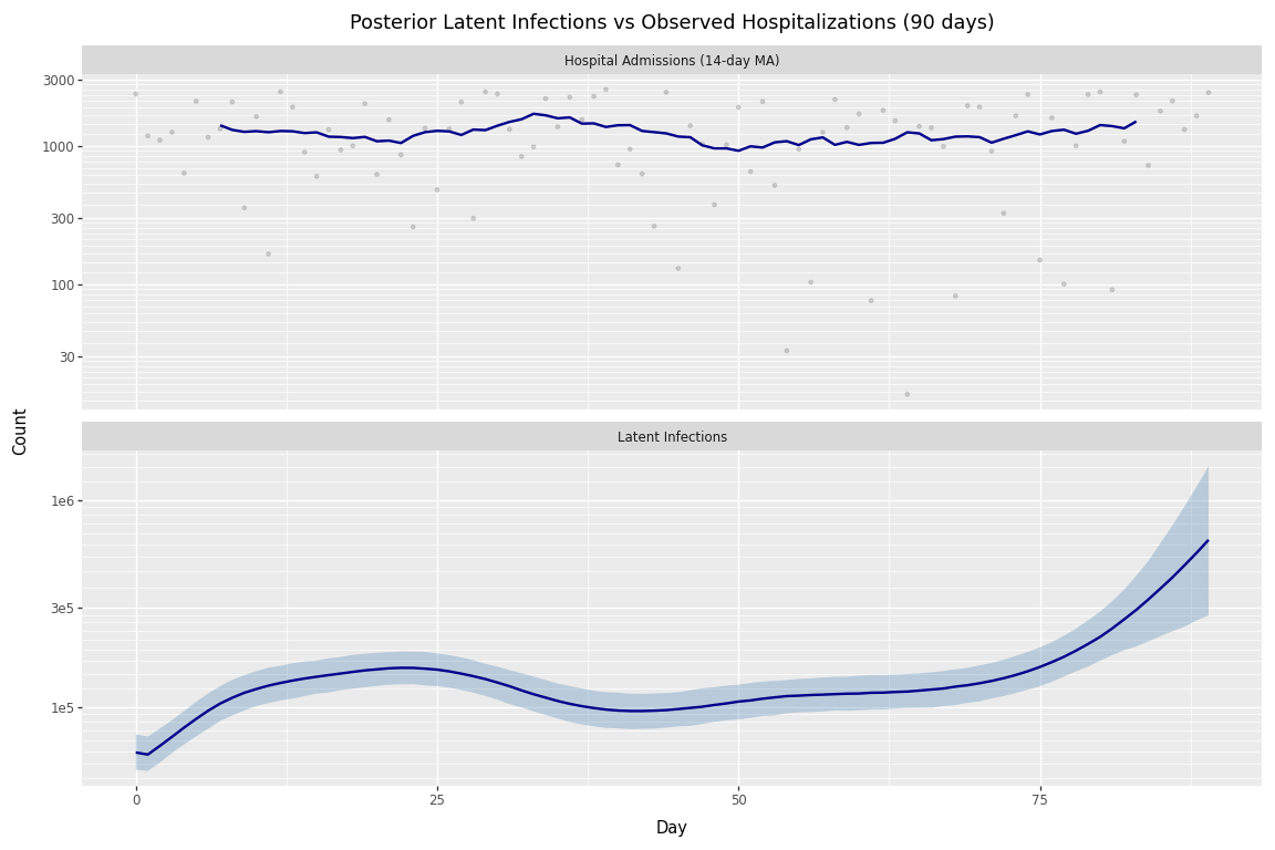
Figure 1: Posterior latent infections and observed hospitalizations (90 days).

Fit: 180 Days

Code

# Clear JAX caches to avoid interference
jax.clear_caches()

n_days_180 = 180
obs_data_180 = prepare_observation_data(
    model, n_days_180, hosp_admits, ca_ww_data, ww_monitored_subpops
)

print(f"Fitting model with {n_days_180} days of data...")
print("  This may take a few minutes...")

start_time = time.time()
model.run(
    num_warmup=1000,
    num_samples=500,
    rng_key=make_rng_key(),
    mcmc_args={"num_chains": 4, "progress_bar": False},
    n_days_post_init=n_days_180,
    population_size=population_size,
    subpop_fractions=subpop_fractions,
    **obs_data_180,
)
# Block until sampling completes for accurate timing
samples_180 = model.mcmc.get_samples()
jax.block_until_ready(samples_180)
elapsed_180 = time.time() - start_time
print(f"Elapsed time: {elapsed_180:.1f} seconds")

Fitting model with 180 days of data...
  This may take a few minutes...
Elapsed time: 404.1 seconds

Code

lat_inf_180 = samples_180["latent_infections"]
print(f"Posterior samples shape: {lat_inf_180.shape}")
print(f"Mean latent infections: {np.mean(lat_inf_180):,.0f}")

Posterior samples shape: (2000, 222)
Mean latent infections: 259,234

We check the model fit, as before.

Code

# ArviZ diagnostics for 180-day fit
samples_180_filtered = filter_samples_for_arviz(
    samples_180, n_init, num_chains=2
)
idata_180 = az.from_dict(posterior=samples_180_filtered)
az.summary(idata_180, var_names=["~latent_infections", "~expected"])

arviz - WARNING - Array contains NaN-value.

	mean	sd	hdi_3%	hdi_97%	mcse_mean	mcse_sd	ess_bulk	ess_tail	r_hat
I0	0.096	0.029	0.044	0.148	0.001	0.001	1332.0	1247.0	1.01
hospital_predicted[0]	1511.033	135.661	1242.752	1749.476	2.948	2.445	2098.0	1889.0	1.00
hospital_predicted[1]	1352.398	117.939	1115.979	1556.397	2.558	2.171	2068.0	1887.0	1.01
hospital_predicted[2]	1212.088	103.739	1024.708	1410.414	2.424	1.945	1748.0	1812.0	1.01
hospital_predicted[3]	1089.425	92.304	924.756	1266.392	2.370	1.748	1459.0	1731.0	1.01
...	...	...	...	...	...	...	...	...	...
ww_site_sd_raw[0]	6.991	0.306	6.446	7.600	0.007	0.006	1826.0	1332.0	1.00
ww_site_sd_raw[1]	7.187	0.349	6.555	7.881	0.007	0.008	2346.0	1468.0	1.00
ww_site_sd_raw[2]	0.299	0.148	0.059	0.568	0.003	0.005	2980.0	1038.0	1.00
ww_site_sd_raw[3]	6.600	0.319	5.975	7.177	0.007	0.007	1864.0	1462.0	1.01
ww_site_sd_raw[4]	6.520	0.414	5.736	7.300	0.009	0.010	2392.0	1415.0	1.00

8170 rows × 9 columns

Code

quantiles_180 = extract_posterior_quantiles(samples_180, n_init, n_days_180)

ci_width_180 = quantiles_180["q95"] - quantiles_180["q05"]
print(f"Posterior summary for {n_days_180} days:")
print(f"  Mean 90% CI width: {ci_width_180.mean():,.0f} infections")
print(f"  Median infections (day 90): {quantiles_180['q50'][90]:,.0f}")

Posterior summary for 180 days:
  Mean 90% CI width: 55,447 infections
  Median infections (day 90): 130,299

Code

# Visualize posterior latent infections and observed hospitalizations (180 days)
infections_df_180 = pd.DataFrame(
    {
        "day": np.arange(n_days_180),
        "median": quantiles_180["q50"],
        "q05": quantiles_180["q05"],
        "q95": quantiles_180["q95"],
        "signal": "Latent Infections",
    }
)

# Add 14-day moving average to smooth noisy daily admissions
hosp_raw_180 = np.array(hosp_admits[:n_days_180], dtype=float)
hosp_ma_180 = (
    pd.Series(hosp_raw_180).rolling(window=14, center=True).mean().values
)

hosp_df_180 = pd.DataFrame(
    {
        "day": np.arange(n_days_180),
        "median": hosp_ma_180,
        "raw": hosp_raw_180,
        "q05": np.nan,
        "q95": np.nan,
        "signal": "Hospital Admissions (14-day MA)",
    }
)

plot_df_180 = pd.concat([infections_df_180, hosp_df_180], ignore_index=True)
plot_df_180["signal"] = pd.Categorical(
    plot_df_180["signal"],
    categories=["Hospital Admissions (14-day MA)", "Latent Infections"],
    ordered=True,
)

(
    p9.ggplot(plot_df_180, p9.aes(x="day"))
    + p9.geom_ribbon(
        p9.aes(ymin="q05", ymax="q95"),
        fill="steelblue",
        alpha=0.3,
    )
    + p9.geom_point(
        p9.aes(y="raw"),
        color="gray",
        alpha=0.3,
        size=1,
    )
    + p9.geom_line(
        p9.aes(y="median"),
        color="darkblue",
        size=1,
    )
    + p9.facet_wrap("~signal", ncol=1, scales="free_y")
    + p9.scale_y_log10()
    + p9.labs(
        x="Day",
        y="Count",
        title="Posterior Latent Infections vs Observed Hospitalizations (180 days)",
    )
    + p9.theme_grey()
    + p9.theme(figure_size=(12, 8))
)

Figure 2: Posterior latent infections and observed hospitalizations (180 days).

Comparing 90-Day vs 180-Day Fits

Comparing the two fits reveals where uncertainty reduction occurs—and why it matters for forecasting.

Code

# Compare CI widths for the overlapping 90-day period
ci_width_90_overlap = quantiles_90["q95"] - quantiles_90["q05"]
ci_width_180_overlap = (
    quantiles_180["q95"][:n_days_90] - quantiles_180["q05"][:n_days_90]
)

# Compute difference in CI widths
ci_diff = ci_width_90_overlap - ci_width_180_overlap
ci_ratio = ci_width_90_overlap / ci_width_180_overlap

print("CI Width Comparison (first 90 days):")
print(
    f"  90-day fit mean CI width:  {ci_width_90_overlap.mean():,.0f} infections"
)
print(
    f"  180-day fit mean CI width: {ci_width_180_overlap.mean():,.0f} infections"
)
print(f"  Mean difference:           {ci_diff.mean():,.0f} infections")
print(f"  Mean ratio (90/180):       {ci_ratio.mean():.2f}x")
print(
    f"\nThe 180-day fit has {(1 - ci_width_180_overlap.mean() / ci_width_90_overlap.mean()) * 100:.1f}% narrower CIs on average"
)

# Per-day comparison
print("\nCI width by time period:")
for start, end, label in [
    (0, 30, "Days 0-30"),
    (30, 60, "Days 30-60"),
    (60, 90, "Days 60-90"),
]:
    mean_90 = ci_width_90_overlap[start:end].mean()
    mean_180 = ci_width_180_overlap[start:end].mean()
    reduction = (1 - mean_180 / mean_90) * 100
    print(
        f"  {label}: 90-day={mean_90:,.0f}, 180-day={mean_180:,.0f}, reduction={reduction:.1f}%"
    )

CI Width Comparison (first 90 days):
  90-day fit mean CI width:  94,167 infections
  180-day fit mean CI width: 47,375 infections
  Mean difference:           46,792 infections
  Mean ratio (90/180):       1.90x

The 180-day fit has 49.7% narrower CIs on average

CI width by time period:
  Days 0-30: 90-day=46,691, 180-day=46,868, reduction=-0.4%
  Days 30-60: 90-day=41,479, 180-day=42,065, reduction=-1.4%
  Days 60-90: 90-day=194,332, 180-day=53,192, reduction=72.6%

Notice that the uncertainty reduction is concentrated in days 60-90—the final month of the 90-day window. Earlier periods (days 0-60) show little change because both fits have sufficient future data to constrain those estimates.

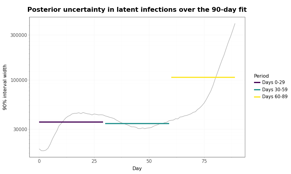
This pattern has a direct implication for forecasting: renewal models are most uncertain at the edge of the observation window. Future observations constrain past latent infections through the renewal equation, but when predicting beyond available data, this constraint disappears. The high uncertainty in days 60-90 of the 90-day fit is exactly what we’d expect when forecasting 30 days ahead—there’s no future signal to anchor the estimates.

Summary

This tutorial demonstrated composing a multi-signal renewal model using PyrenewBuilder:

Configure latent process (configure_latent): generation interval, initial infections, temporal dynamics
Add observation processes (add_observation): each declares its infection resolution and gets a name for data binding
Build and run (build, model.run): the model routes infections to observations based on resolution and runs NUTS inference

Key Concepts

Two-part structure: Renewal models separate latent infection dynamics from observation processes
Infection resolution: Observation processes declare whether they need aggregate or subpop-level infections
Data routing: PyrenewBuilder automatically routes infection trajectories to the appropriate observation processes
Time alignment: Observations must be offset by n_initialization_points to align with model time

Next Steps

Explore different temporal processes for \(\mathcal{R}(t)\) in the Hierarchical Latent Infections tutorial
Learn about count-based observation models in Observation Processes: Counts
Learn about continuous measurement models in Observation Processes: Measurements

Building Multi-Signal Renewal Models

Overview

Related Tutorials

What This Tutorial Covers

Model Structure

Infection Resolution

Latent Infection Process

Generation Interval

I0: Initial Infections

Initial Log Rt

Temporal Processes for \(\mathcal{R}(t)\)

Observation Processes

Signal Naming

Hospital Admissions

Wastewater Concentrations

Wastewater Observation Process

Wastewater Data

Model Building

Configuring the Latent Process

Specifying the Observation Processes, Data

Fitting the Model to Data: model.run()

Shared Time Axis

Observation Data by Signal Type

Jurisdiction-level signals (dense)

Subpopulation-level signals (sparse)

Population Structure

Example model.run() Call

Running the Model

Fit: 90 Days

Fit: 180 Days

Comparing 90-Day vs 180-Day Fits

Summary

Key Concepts

Next Steps

Fitting the Model to Data: `model.run()`

Example `model.run()` Call