Simulation-based calibration of Bayesian NBBP model

Theory

One sanity check of a Bayesian model implementation is simulation-based calibration. We simulate from a model by drawing a dataset from the prior predictive distribution. Then we fit the model and check whether the true value was covered at many quantiles. If we repeat this process enough times, the percentage of true values covered at the $x$th percentile should be $x$. That is, when we draw from the prior predictive, the posterior should obey frequentist coverage properties.

We can also examine how well point estimates (say, the posterior mean) recapitulate the truth along the way.

This is a best-case sort of test, the results of which come with the package as data.

Main results

The coverage at the 1st through 99th percentiles is available as sbc_quants.

Here are the results for $R$:

library(nbbp)
library(ggplot2)
data(sbc_quants)

sbc_quants |>
  ggplot(aes(x = quantile, y = r_covered)) +
  theme_minimal() +
  geom_point() +
  geom_abline(intercept = 0, slope = 1, col = "red") +
  xlab("Quantile") +
  ylab("Observed coverage of R at quantile")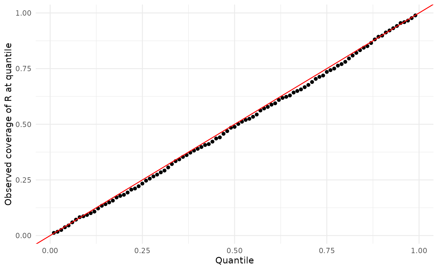

Here are the results for $k$:

library(ggplot2)
data(sbc_quants)

sbc_quants |>
  ggplot(aes(x = quantile, y = k_covered)) +
  theme_minimal() +
  geom_point() +
  geom_abline(intercept = 0, slope = 1, col = "red") +
  xlab("Quantile") +
  ylab("Observed coverage of k at quantile")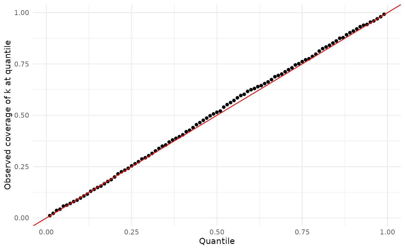

Ancillary results

Also available (as data(sbc_ests)) is information about posterior and MCMC quality.

Estimating $R$

Here we plot the posterior median $R$ against the true simulating $R$, with the 95% CI as a bar. Points are red (with non-transparent bars) when the true value is not in the 95% CI, and blue (with transparent bars) otherwise.

data(sbc_ests)

sbc_ests |>
  dplyr::mutate(covered = dplyr::case_when(
    r_true >= r_low & r_true <= r_high ~ TRUE,
    .default = FALSE
  )) |>
  ggplot(aes(
    x = r_true, y = r_point,
    ymin = r_low, ymax = r_high,
    col = covered,
  )) +
  theme_minimal() +
  geom_abline(intercept = 0, slope = 1, col = "grey", lty = 2, lwd = 2) +
  geom_errorbar(aes(alpha = 1 - covered), show.legend = FALSE) +
  geom_point() +
  xlab("true R") +
  ylab("estimated R") +
  scale_x_continuous(trans = "log") +
  scale_y_continuous(trans = "log")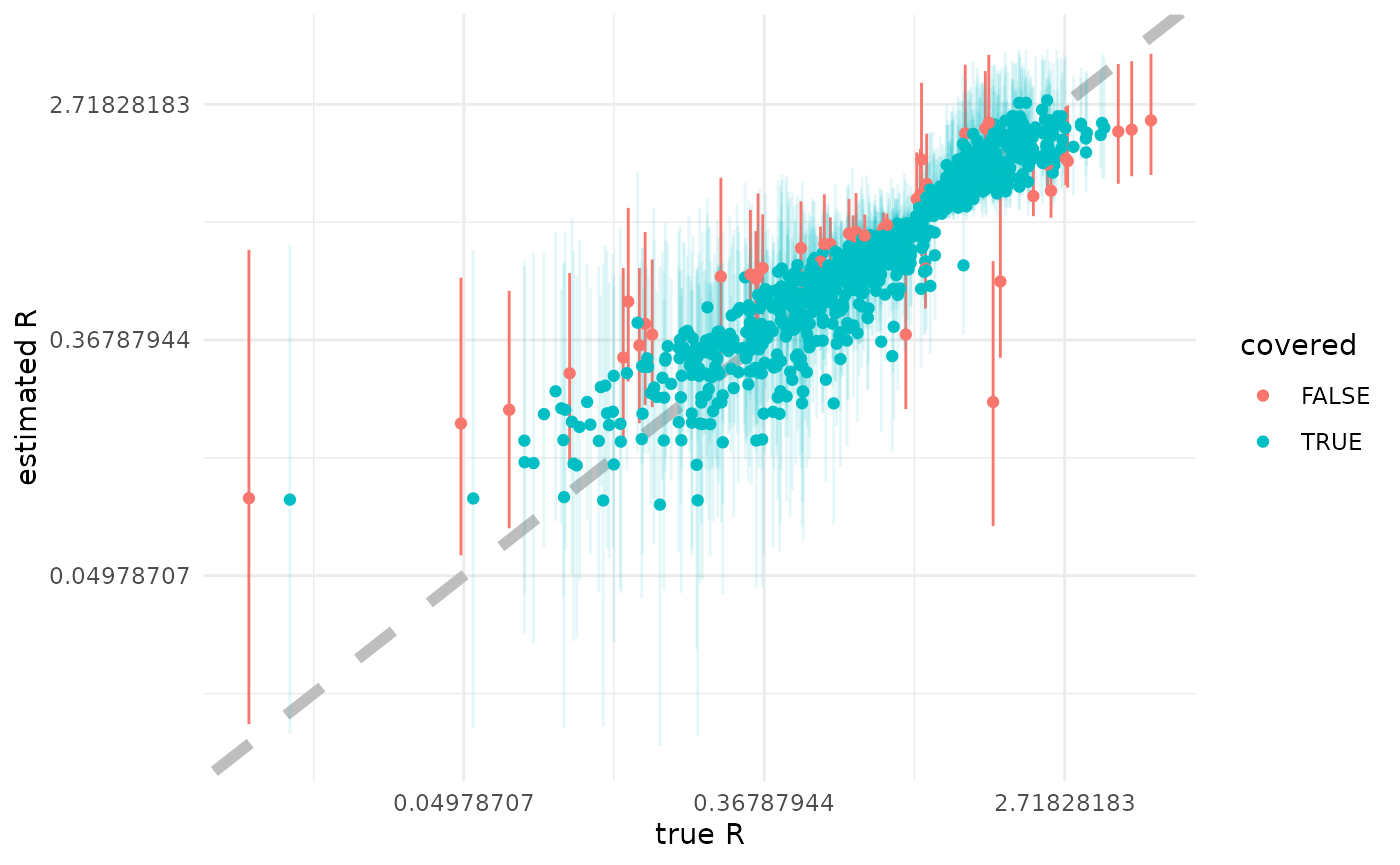

Estimating $k$

Here we plot the posterior median $k$ against the true simulating $k$, with the 95% CI as a bar. Points are red (with non-transparent bars) when the true value is not in the 95% CI, and blue (with transparent bars) otherwise.

data(sbc_ests)

sbc_ests |>
  dplyr::mutate(covered = dplyr::case_when(
    k_true >= k_low & k_true <= k_high ~ TRUE,
    .default = FALSE
  )) |>
  ggplot(aes(
    x = k_true, y = k_point,
    ymin = k_low, ymax = k_high,
    col = covered,
  )) +
  theme_minimal() +
  geom_abline(intercept = 0, slope = 1, col = "grey", lty = 2, lwd = 2) +
  geom_errorbar(aes(alpha = 1 - covered), show.legend = FALSE) +
  geom_point() +
  xlab("true k") +
  ylab("estimated k") +
  scale_x_continuous(trans = "log") +
  scale_y_continuous(trans = "log")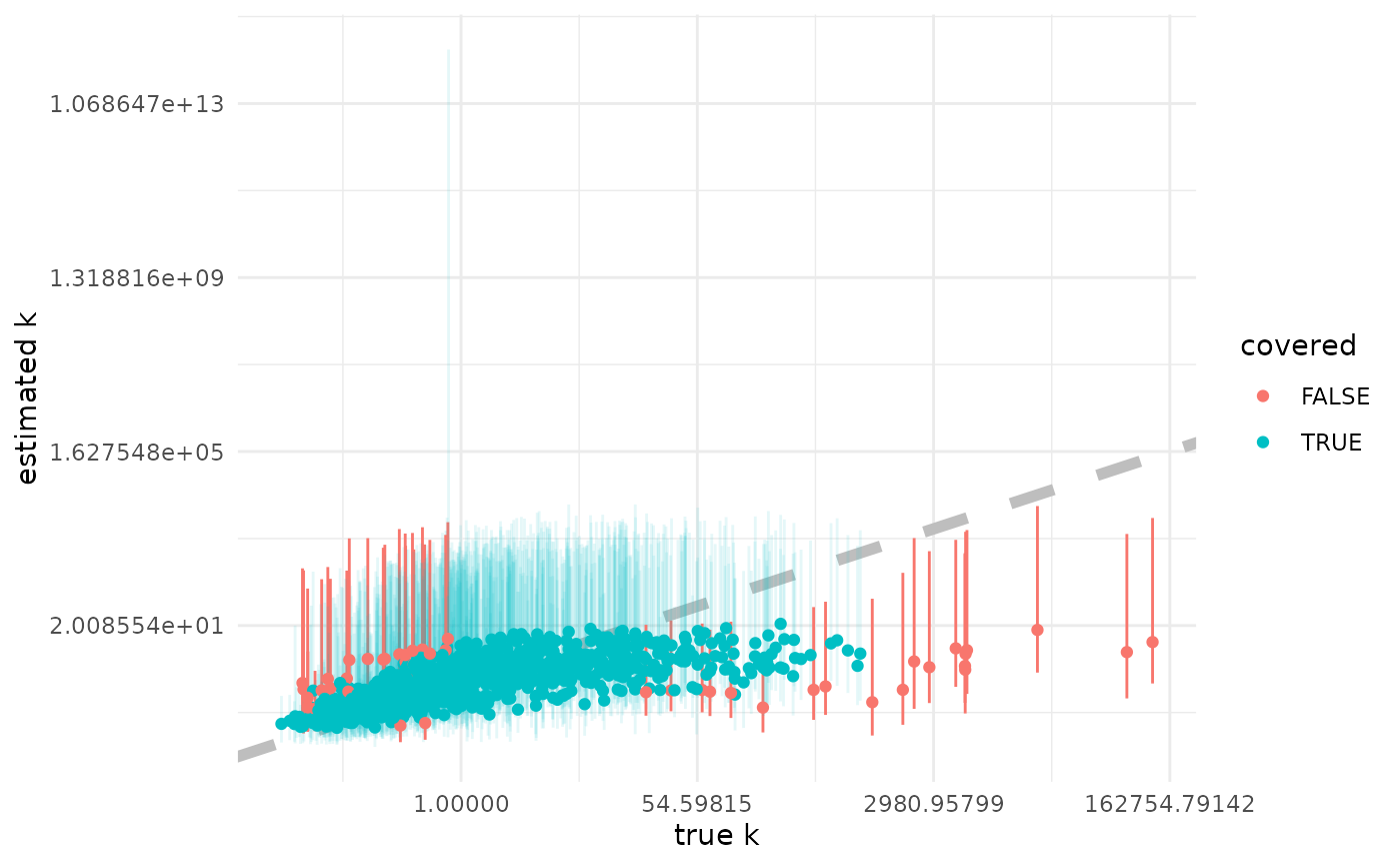

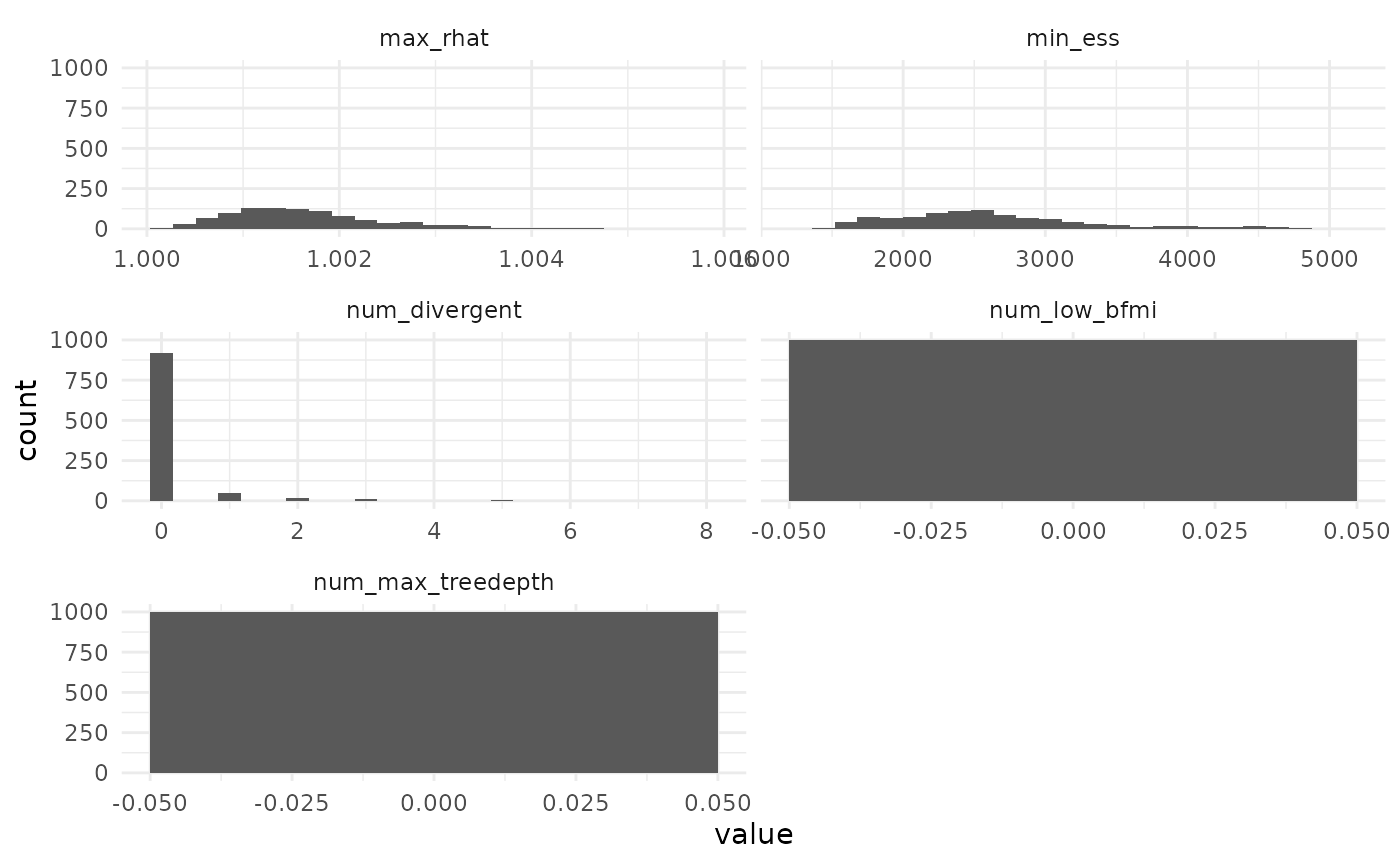
MCMC behavior

We can also see that most MCMC performed well, with a few exceptions that are visible mostly through the limits chosen for the axes when we plot all the diagnostics.

sbc_ests |>
  dplyr::select(c("min_ess", "max_rhat", "num_low_bfmi", "num_divergent", "num_max_treedepth")) |>
  dplyr::mutate(index = dplyr::row_number()) |>
  tidyr::pivot_longer(!index) |>
  dplyr::select(!index) |>
  ggplot(aes(x = value)) +
  theme_minimal() +
  geom_histogram(bins = 25) +
  facet_wrap(~name, ncol = 2, scales = "free_x")

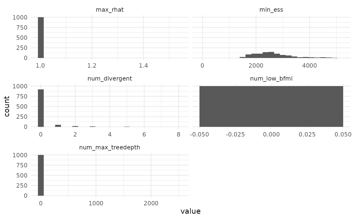
Filtering for large n_eff and small Rhat, as was done to obtain the quantiles in sbc_quants removes the runs with pathologically bad num_max_treedepth as well.

sbc_ests |>
  dplyr::filter(min_ess > 1000 | max_rhat < 1.005) |>
  dplyr::select(c("min_ess", "max_rhat", "num_low_bfmi", "num_divergent", "num_max_treedepth")) |>
  dplyr::mutate(index = dplyr::row_number()) |>
  tidyr::pivot_longer(!index) |>
  dplyr::select(!index) |>
  ggplot(aes(x = value)) +
  theme_minimal() +
  geom_histogram(bins = 25) +
  facet_wrap(~name, ncol = 2, scales = "free_x")