nbbp

Welcome to nbbp, an R package for inference of parameters of negative binomial branching process models from final outbreak size data. This vignette covers the basics of inferring parameters from simple data, where every possible chain size is observable and every observed chain size is known exactly. More advanced forms of data are covered in the “Advanced data” vignette. Note that a “chain” is not necessarily a linear structure and includes transmission trees. That is, it consists of the first infected individual, any and all individuals infected by the first, any and all individuals infected by the second generation, and so forth. But as we are working with the final size of a chain, each observation is simply an integer: the total number of infections, including the first.

As our example, we will analyze Borealpox. Currently, there are seven singleton cases which have been observed, each corresponding to a final chain size of 1. The data is included in the package, though we could have simply made it ourselves (e.g. rep(1, 7)).

library(nbbp)
library(ggplot2)
data(borealpox)

borealpox

## [1] 1 1 1 1 1 1 1

Simple Bayesian inference

Fitting the model is accomplished by passing the data and the model object to fit_nbbp_homogenous_bayes(), which internally uses rstan for inference. This function allows significant control over rstan settings, as well as adjustments to the default priors (for more on those, see the vignette “Default priors”). Here, for reproducibility, we will set the random seed, so that any time we run this code (with the same version of rstan) we will get the same answer.

fit <- fit_nbbp_homogenous_bayes(
  all_outbreaks = borealpox,
  seed = 42
)

The output is a regular rstan::stanfit object, and can be summarized in the usual ways. As we are performing Bayesian inference, we should always check convergence diagnostics. (For more on so doing, see the stan manual, the rstan reference, or Chapter 11.4 in Bayesian Data Analysis.)

rstan::check_hmc_diagnostics(fit)

## 
## Divergences:

## 0 of 10000 iterations ended with a divergence.

## 
## Tree depth:

## 0 of 10000 iterations saturated the maximum tree depth of 10.

## 
## Energy:

## E-BFMI indicated no pathological behavior.

rstan::summary(fit)$summary[, c("n_eff", "Rhat")]

##                        n_eff     Rhat
## r_eff               2258.851 1.000824
## inv_sqrt_dispersion 2614.954 1.001077
## dispersion          9478.288 1.000022
## exn_prob            3325.017 1.000598
## p_0                 4546.211 1.000603
## lp__                1852.968 1.002097

Now that we can see our MCMC is trustworthy, we can look at what our results are. There are 5 variables tracked in the object. Primarily, we have $R$ (r_eff) and $k$ (dispersion). Additionally, we track two values which are functions of $R$ and $k$ but can be useful in their own right. These are the probability that a chain goes extinct (exn_prob) and the probability that any one infection produces no additional infections (p_0). As it is the native parameter of the model, we also have $1 / \sqrt{k}$ (inv_sqrt_dispersion)

Let us see what we have estimated.

fit

## Inference for Stan model: nbbp_homogenous.
## 4 chains, each with iter=5000; warmup=2500; thin=1; 
## post-warmup draws per chain=2500, total post-warmup draws=10000.
## 
##                         mean  se_mean         sd  2.5%   25%   50%   75%  97.5%
## r_eff                   0.47     0.01       0.43  0.05  0.18  0.34  0.61   1.67
## inv_sqrt_dispersion     1.75     0.02       1.10  0.09  0.85  1.67  2.52   4.03
## dispersion          14966.82 14768.94 1437852.61  0.06  0.16  0.36  1.38 118.09
## exn_prob                0.99     0.00       0.03  0.89  1.00  1.00  1.00   1.00
## p_0                     0.80     0.00       0.10  0.57  0.74  0.81  0.87   0.96
## lp__                   -5.87     0.03       1.15 -8.91 -6.34 -5.53 -5.04  -4.71
##                     n_eff Rhat
## r_eff                2259    1
## inv_sqrt_dispersion  2615    1
## dispersion           9478    1
## exn_prob             3325    1
## p_0                  4546    1
## lp__                 1853    1
## 
## Samples were drawn using NUTS(diag_e) at Tue May 20 20:00:40 2025.
## For each parameter, n_eff is a crude measure of effective sample size,
## and Rhat is the potential scale reduction factor on split chains (at 
## convergence, Rhat=1).

We can see that the model is relatively confident $R < 1$, but there is still considerable uncertainty about its value. We can see even greater uncertainty about $k$, which is typical in practice without a relatively large number of chains observed.

While rstan provides some basic plotting capabilities, this is not the only way to do so. Here we extract and plot things ourselves directly with ggplot, though we could also use the bayesplot package which has many nice visualizations. Plots show us

par_df <- rstan::extract(fit, pars = c("r_eff", "dispersion", "p_0", "exn_prob")) |>
  as.data.frame()

par_df |>
  ggplot(aes(x = r_eff, y = after_stat(density))) +
  geom_histogram() +
  theme_minimal() +
  xlab("R")

## `stat_bin()` using `bins = 30`. Pick better value with `binw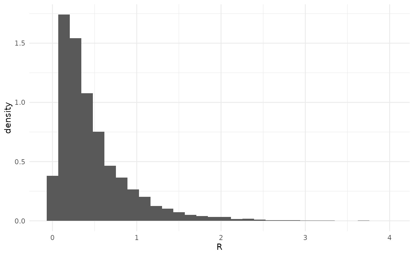idth`.

Here we can see that the posterior density is greatest for small values of $R$, as well as the long tails with larger values.

The uncertainty about the dispersion parameter often makes it more usefully considered on the log-scale.

par_df |>
  ggplot(aes(x = log(dispersion), y = after_stat(density))) +
  geom_histogram() +
  theme_minimal() +
  xlab("log(k)")

## `stat_bin()` using `bins = 30`. Pick better value with `binw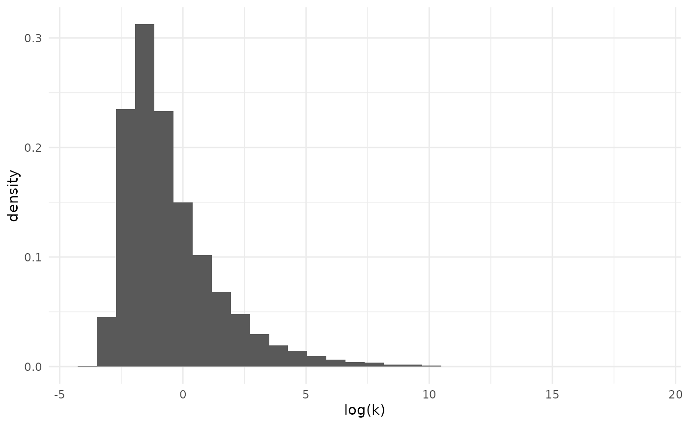idth`.

This shows us that, while there is considerable uncertainty, the model favors relatively strong overdispersion.

The probability that a chain goes extinct (exn_prob) is a function of $R$ and $k$.

par_df |>
  ggplot(aes(x = exn_prob, y = after_stat(density))) +
  geom_histogram() +
  theme_minimal() +
  xlab("extinction probability")

## `stat_bin()` using `bins = 30`. Pick better value with `binw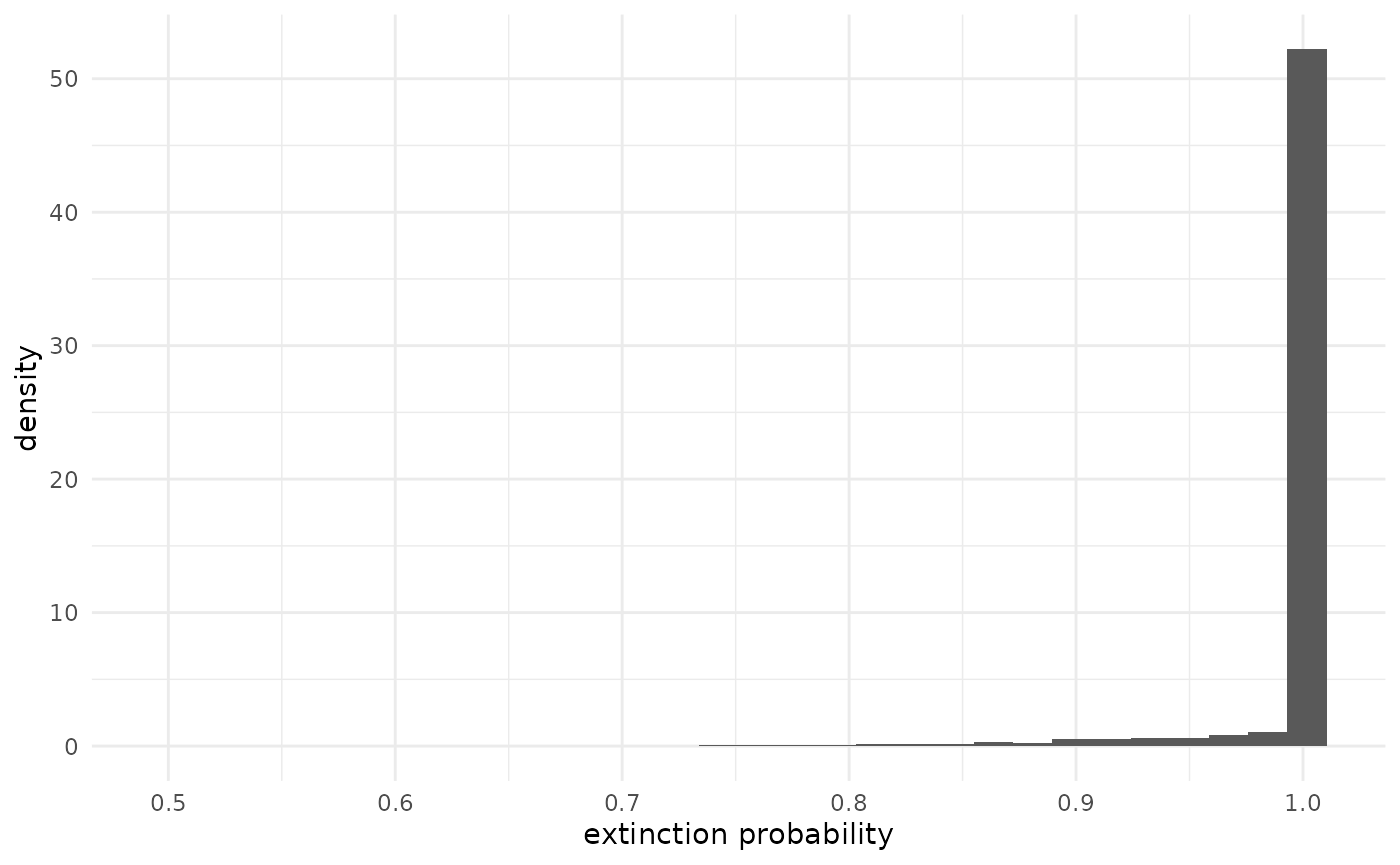idth`.

It is always 1 when $R < 1$, so since there is a 89% probability that $R < 1$, most of the prior mass is on 1 exactly. Most of the rest of the mass is on values near 1, but we can see the considerably uncertainty about $R$ and $k$ manifest in the long left tail. While it isn’t probable that 7 chains went extinct if the extinction probability is only, say, 0.8, it is not impossible ($0.8^7 \approx 0.21$).

The probability of 0 offspring (p_0) is also a function of $R$ and $k$, and measures the probability that any particular infection produces no more infections.

par_df |>
  ggplot(aes(x = p_0, y = after_stat(density))) +
  geom_histogram() +
  theme_minimal() +
  xlab("probability of 0 offspring")

## `stat_bin()` using `bins = 30`. Pick better value with `binw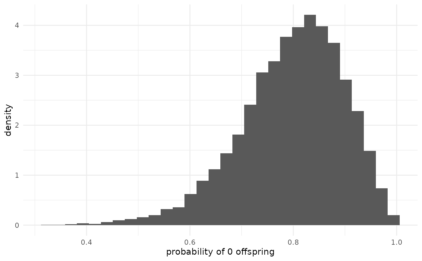idth`.

Since we have not seen any chains produce offspring, we should not be surprised to see that this probability is near 1. (When there is strong overdispersion (small $k$), this can be near 1 even when $R$ is above 1.) We might expect, since none of these cases have produced any offspring, that the posterior would have a mode at 1. However, the default priors pull towards regimes where this probability is smaller (larger $R$ and $k$ both make it more likely that an infection has offspring), as can be seen in the plot in the “Default priors” vignette.

Simple maximum likelihood inference

The package also supports maximum likelihood inference. We do not suggest using maximum likelihood as the primary form of inference, but sometimes one may wish to see the results. This can be accomplished with fit_nbbp_homogenous_ml() which has much the same interface as fit_nbbp_homogenous_bayes(). By default, this attempts to obtain 10 converged search replicates from random starting locations, and will adaptively determine an appropriate method for producing confidence intervals.

fit_ml <- fit_nbbp_homogenous_ml(
  all_outbreaks = borealpox,
  seed = 42,
  ci_width = 0.95
)

The object returned here is a slightly enriched version of what is returned by rstan::optimizing for the replicate search which produced the maximum maximized likelihood.

fit_ml

## $par
##               r_eff inv_sqrt_dispersion          dispersion            exn_prob 
##        6.770924e+00        2.411232e+05        1.719975e-11        1.000000e+00 
##                 p_0 
##        1.000000e+00 
## 
## $value
## [1] -3.214485e-09
## 
## $return_code
## [1] 0
## 
## $theta_tilde
##         r_eff inv_sqrt_dispersion   dispersion exn_prob p_0
## [1,] 6.770924            241123.2 1.719975e-11        1   1
## 
## $convergence
##                          min           max
## log_likelihood -9.587682e-09 -3.214485e-09
## r_eff           7.471339e-10  5.889395e+01
## dispersion      1.609900e-11  1.352528e+05
## 
## $ci
##                   2.5%       97.5%
## r_eff      7.63948e-10    42.56584
## dispersion 1.45387e-11 73516.09755
## 
## $ci_method
## [1] "hybrid(parametric_bootstrap)"

Here, $par tells us our maximum likelihood estimates of the parameters (and the additionally-tracked variables), and $ci the confidence intervals (for only $R$ and $k$). Additionally, $convergence returns the range of values of $R$, $k$, and the maximized likelihood across all search replicates. When there are wide (relative to the value) ranges observed, this signals trouble.

Sometimes, we can understand the nature of issues with maximum likelihood inference by examining the likelihood surface. The function compute_likelihood_surface() computes this at a grid and enables visualization.

r_vec <- exp(seq(log(1e-4), log(2), length.out = 100))
k_vec <- exp(seq(log(0.01), log(9999), length.out = 100))

lnl_surface <- compute_likelihood_surface(
  borealpox,
  r_grid = r_vec,
  k_grid = k_vec
)

lnl_surface |>
  ggplot(aes(x = r, y = k, fill = log_dens)) +
  theme_minimal() +
  geom_tile() +
  scale_x_continuous(trans = "log") +
  scale_y_continuous(trans = "log") +
  xlab("R") +
  scale_fill_viridis_c(option = "magma")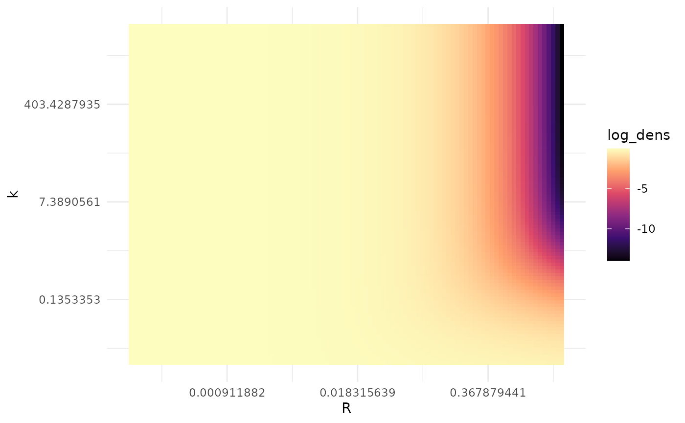

Roughly speaking, by Wilks’ theorem the region where the log-likelihood is within 12 units of the maximum value is within a bivariate 95% confidence region. We can see there is extensive uncertainty here, as most of this plot is within a 12 log-likelihood unit range of the maximum.

We also see that the the log-likelihood surface does not appear to have a single mode. It is easier to see what is going on if we focus in on where the likelihood is highest: small values of $R$.

r_vec <- exp(seq(log(1e-4), log(0.02), length.out = 100))

lnl_surface <- compute_likelihood_surface(
  borealpox,
  r_grid = r_vec,
  k_grid = k_vec
)

lnl_surface |>
  ggplot(aes(x = r, y = k, fill = log_dens)) +
  theme_minimal() +
  geom_tile() +
  scale_x_continuous(trans = "log") +
  scale_y_continuous(trans = "log") +
  xlab("R") +
  scale_fill_viridis_c(option = "magma")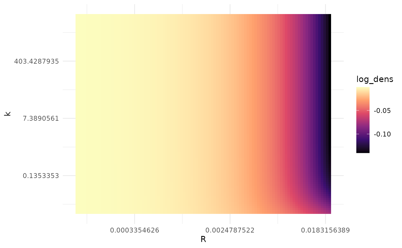

The likelihood increases as $R$ decreases, but once $R$ gets small, for a fixed $R$ the likelihood appears to be constant in $k$. The presence of this ridge shape, rather than a single mode, likely explains the convergence difficulties we saw with maximum likelihood estimation. For sufficiently small $R$, we can pick any $k$ and not change the likelihood, so the value of $k$ the optimizer ends up giving us is going to depend a lot on where it started.

“Is $R$ different?”

While inference in this package is focused on cases where $R$ is homogenous, we can still try to make comparisons about $R$ between scenarios.

Measles

For example, we might ask if $R$ is different in the two measles datasets included in the package. These correspond to cases in the United States from 1997-1999 and Canada from 1998-2001. To investigate this, we can simply fit the model, separately, to both datasets and examine the posteriors.

data(measles_us_97)
data(measles_canada_98)

us <- fit_nbbp_homogenous_bayes(measles_us_97, iter = 5000, seed = 42)
canada <- fit_nbbp_homogenous_bayes(measles_canada_98, iter = 5000, seed = 42)

We have two sets of MCMC convergence diagnostics to check now.

rstan::check_hmc_diagnostics(us)

## 
## Divergences:

## 0 of 10000 iterations ended with a divergence.

## 
## Tree depth:

## 0 of 10000 iterations saturated the maximum tree depth of 10.

## 
## Energy:

## E-BFMI indicated no pathological behavior.

rstan::summary(us)$summary[, c("n_eff", "Rhat")]

##                        n_eff      Rhat
## r_eff               5358.979 1.0005487
## inv_sqrt_dispersion 6294.843 0.9997029
## dispersion          4576.889 0.9999844
## exn_prob                 NaN       NaN
## p_0                 6285.057 0.9998974
## lp__                4028.536 1.0011858

We would normally be troubled by a NaN. However, when the posterior probability that $R < 1$ is 1, the extinction probability is always 1. Convergence diagnostics make use of the variance of a quantity in the posterior, and therefore produce NaNs here.

rstan::check_hmc_diagnostics(canada)

## 
## Divergences:

## 0 of 10000 iterations ended with a divergence.

## 
## Tree depth:

## 0 of 10000 iterations saturated the maximum tree depth of 10.

## 
## Energy:

## E-BFMI indicated no pathological behavior.

rstan::summary(canada)$summary[, c("n_eff", "Rhat")]

##                        n_eff     Rhat
## r_eff               4245.724 1.000902
## inv_sqrt_dispersion 4998.830 1.000269
## dispersion          2741.696 1.001163
## exn_prob            4062.062 1.001739
## p_0                 4675.906 1.000146
## lp__                3855.287 1.000061

r_df <- data.frame(
  r = c(
    unlist(rstan::extract(us, "r_eff")),
    unlist(rstan::extract(canada, "r_eff"))
  ),
  location = c(
    rep("US", 10000),
    rep("Canada", 10000)
  )
)

r_df |>
  ggplot(aes(x = r, fill = location, y = after_stat(density))) +
  geom_histogram(position = "identity", alpha = 0.7) +
  theme_minimal() +
  xlab("R")

## `stat_bin()` using `bins = 30`. Pick better value with `binw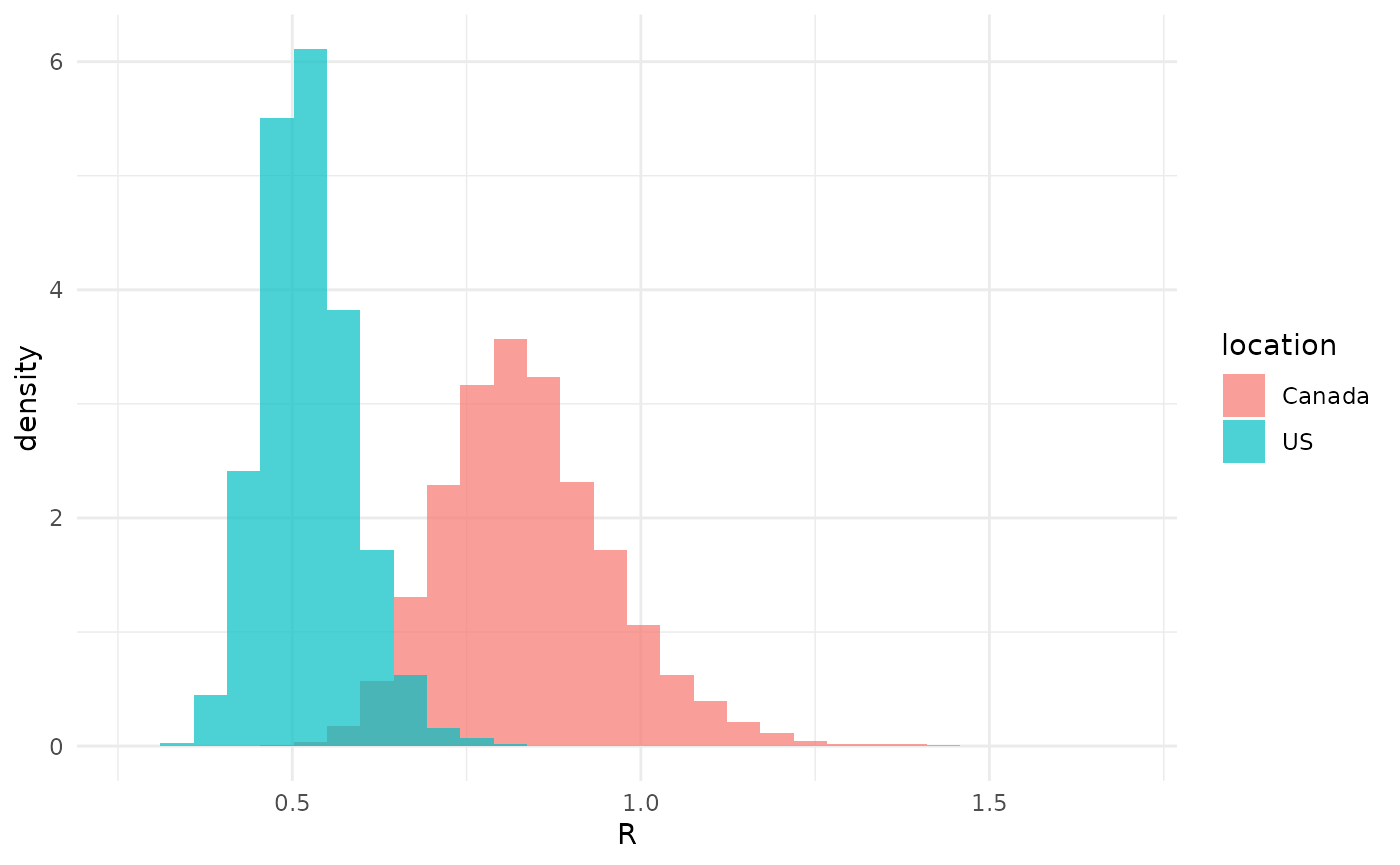idth`.

The posterior distributions on $R$ exhibit rather low overlap, suggesting that $R$ is in fact different.

We can quantify this, if we like, by some measure of overlap of the posteriors. We might, for example, contemplate what percent of the posterior on $R_{\text{US}}$ is above the 2.5th percentile of the posterior on $R_{\text{Canada}}$. We would then compute the 2.5th percentile of $R_{\text{Canada}}$, find that it is 0.63, and count the percent of samples of $R_{\text{US}}$ which are larger than this and find that it is 6%. Or we could do this the other way around, and ask what percent of the posterior on $R_{\text{Canada}}$ is below below the 97.5th percentile of the posterior on $R_{\text{US}}$. This is 5%.

These summaries are not entirely satisfying, as we have both an arbitrary reference quantile and an asymmetric measure. We could instead try to define, jointly, a single probability $\alpha$ and corresponding quantile $q$ such that $\text{Pr}(R_{\text{US}} > q \mid \text{data}) = \text{Pr}(R_{\text{Canada}} \leq q \mid \text{data}) = \alpha$. That is, find the value of $R$ for which the posterior probability that $R_{\text{US}}$ is larger is equal to the posterior probability that $R_{\text{Canada}}$ is smaller. Since $\text{Pr}(R_{\text{US}} \leq q \mid \text{data}) = 1 - \text{Pr}(R_{\text{US}} > q \mid \text{data})$, we can rearrange this equation and remove $\alpha$, simply writing $\text{Pr}(R_{\text{US}} \leq q \mid \text{data}) + \text{Pr}(R_{\text{Canada}} \leq q \mid \text{data}) = 1$. Once we solve for $q$, we get our overlap percent ($\alpha \times 100$%) for free and can estimate it from our samples of either the posterior on $R_{\text{US}}$ or on $R_{\text{Canada}}$. This can’t simply be done in one chain of dplyr calls, so we will need to write some code.

find_overlap <- function(r_small, r_large) {
  # As pointed out, ECDFs are more efficient
  # https://stats.stackexchange.com/questions/122857/how-to-determine-overlap-of-two-empirical-distribution-based-on-quantiles #nolint
  p_r_small <- stats::ecdf(r_small)
  p_r_large <- stats::ecdf(r_large)
  loss_fn <- function(q) {
    ((p_r_small(q) + p_r_large(q)) - 1)^2
  }
  optimize(loss_fn, range(c(r_small, r_large)))$minimum
}

q <- find_overlap(
  r_df |> dplyr::filter(location == "US") |> dplyr::pull(r),
  r_df |> dplyr::filter(location == "Canada") |> dplyr::pull(r)
)

overlap <- 1.0 - mean(
  r_df |>
    dplyr::filter(location == "US") |>
    dplyr::pull(r)
  <= q
)

This gives us an overlap of 4%.

MERS-CoV

As another example, we might ask if $R$ is different for MERS-CoV in the Arabian Peninsula after June 1, 2013 (compared to before). Again, we fit both datasets separately and compare.

data(mers_pre_june)
data(mers_post_june)

before <- fit_nbbp_homogenous_bayes(mers_pre_june, iter = 5000, seed = 42)
after <- fit_nbbp_homogenous_bayes(mers_post_june, iter = 5000, seed = 42)

Again we have two sets of MCMC convergence diagnostics to check.

rstan::check_hmc_diagnostics(before)

## 
## Divergences:

## 0 of 10000 iterations ended with a divergence.

## 
## Tree depth:

## 0 of 10000 iterations saturated the maximum tree depth of 10.

## 
## Energy:

## E-BFMI indicated no pathological behavior.

rstan::summary(before)$summary[, c("n_eff", "Rhat")]

##                        n_eff     Rhat
## r_eff               2961.937 1.000446
## inv_sqrt_dispersion 3475.358 1.000534
## dispersion          3149.092 1.000688
## exn_prob            2856.461 1.000584
## p_0                 4900.390 1.000125
## lp__                2261.079 1.001697

rstan::check_hmc_diagnostics(after)

## 
## Divergences:

## 0 of 10000 iterations ended with a divergence.

## 
## Tree depth:

## 0 of 10000 iterations saturated the maximum tree depth of 10.

## 
## Energy:

## E-BFMI indicated no pathological behavior.

rstan::summary(after)$summary[, c("n_eff", "Rhat")]

##                        n_eff     Rhat
## r_eff               2271.476 1.000319
## inv_sqrt_dispersion 2587.110 1.000519
## dispersion          2345.970 1.001626
## exn_prob            2644.302 1.000898
## p_0                 4597.428 1.000400
## lp__                1385.952 1.000513

r_df <- data.frame(
  r = c(
    unlist(rstan::extract(before, "r_eff")),
    unlist(rstan::extract(after, "r_eff"))
  ),
  time = c(
    rep("before", 10000),
    rep("after", 10000)
  )
)

r_df |>
  ggplot(aes(x = r, fill = time, y = after_stat(density))) +
  geom_histogram(position = "identity", alpha = 0.7) +
  theme_minimal() +
  xlab("R")

## `stat_bin()` using `bins = 30`. Pick better value with `binw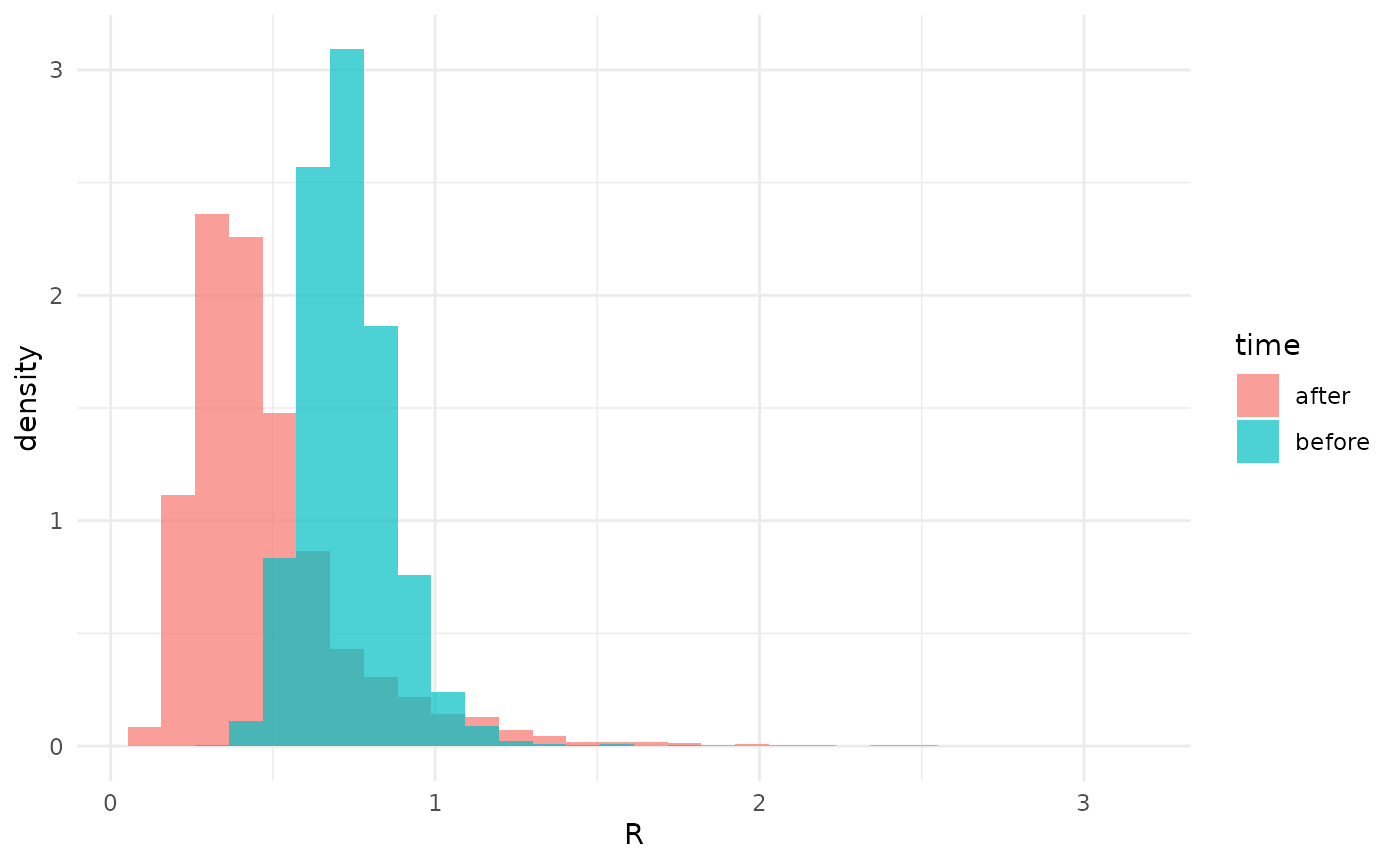idth`.

The posterior for the later cases completely covers the posterior for the earlier ones. Clearly, there is no evidence for a difference in $R$.