Advanced data • nbbp

In the first vignette, we considered only examples where we could observe every chain size exactly, both in theory and in practice. This is not always true. Some times we only consider chains that have at least some number of cases, and some times we only know that a chain was at least a given size. Our investigation of these topics will use data on outbreaks of the pneumonic plague reported by Nishiura et al. (2012).

library(nbbp)
library(dplyr)

## 
## Attaching package: 'dplyr'

## The following objects are masked from 'package:stats':
## 
##     filter, lag

## The following objects are masked from 'package:base':
## 
##     intersect, setdiff, setequal, union

library(ggplot2)
data(pneumonic_plague)
summary(pneumonic_plague)

##    Min. 1st Qu.  Median    Mean 3rd Qu.    Max. 
##     2.0     4.5    12.0   277.6    24.0  5009.0

Conditioning on observable chain sizes

Among the data, we see a number of relatively small chains, but no singletons. This is because when Nishiura et al. investigated outbreaks of the pneumonic plague they compiled data only on chains of at least 2 cases.

In general, any particular dataset may include chains only if they reach some minimum size threshold. Analyzing such data requires appropriately conditioning the likelihood using the condition_geq argument. For analyzing the pneumonic plague data, we need to set condition_geq = rep(2, 19), indicating that for each of the 19 chains in the dataset, the minimum observation size was 2. While it is generally expected that condition_geq = rep(minimum_observation_size, number_of_chains), by specifying the minimum observation size for each chain separately, it is possible to combine datasets collected according to different standards in a unified interface. One more wrinkle remains before analysis.

What if the chain didn’t go extinct?

We might also notice in that data that there is one very large chain of size 5009. This is not a stuttering chain. Nishiura et al. call it a major epidemic. We have two choices for how to appropriately handle this. Both amount to acknowledging that this chain did not go extinct due to any feature of the branching process model that this package uses, but differ in how they treat it.

Treat it as non-extinct

We can simply declare that this chain did not go extinct. Mathematically this requires partitioning outcomes into extinct and non-extinct chains and considering them separately. But in practice with nbbp this is done by declaring the size of a chain to be Inf (which is the package’s shorthand for non-extinct). Note that this will force $R > 1$ because when $R < 1$ every chain must go extinct.

pneumonic_plague_inf <- pneumonic_plague
pneumonic_plague_inf[4] <- Inf

fit_inf <- fit_nbbp_homogenous_bayes(
  all_outbreaks = pneumonic_plague_inf,
  condition_geq = rep(2, length(pneumonic_plague)),
  seed = 42
)

As always, first we inspect the MCMC.

rstan::check_hmc_diagnostics(fit_inf)

## 
## Divergences:

## 31 of 10000 iterations ended with a divergence (0.31%).
## Try increasing 'adapt_delta' to remove the divergences.

## 
## Tree depth:

## 0 of 10000 iterations saturated the maximum tree depth of 10.

## 
## Energy:

## E-BFMI indicated no pathological behavior.

rstan::summary(fit_inf)$summary[, c("n_eff", "Rhat")]

##                        n_eff      Rhat
## r_eff               2146.353 1.0003360
## inv_sqrt_dispersion 2652.047 1.0004340
## dispersion          5387.564 1.0003586
## exn_prob            5569.015 0.9999126
## p_0                 2690.675 1.0005069
## lp__                2052.369 1.0018124

We see a small number of divergent transitions, but things look good on the whole.

Now we can look at what we estimated.

fit_inf

## Inference for Stan model: nbbp_homogenous.
## 4 chains, each with iter=5000; warmup=2500; thin=1; 
## post-warmup draws per chain=2500, total post-warmup draws=10000.
## 
##                         mean  se_mean         sd   2.5%    25%    50%    75%
## r_eff                   1.09     0.00       0.09   1.01   1.04   1.07   1.12
## inv_sqrt_dispersion     1.42     0.02       1.08   0.05   0.54   1.18   2.10
## dispersion          33083.02 32095.87 2355837.36   0.06   0.23   0.72   3.43
## exn_prob                0.94     0.00       0.04   0.84   0.92   0.95   0.97
## p_0                     0.54     0.00       0.15   0.35   0.40   0.52   0.67
## lp__                  -79.08     0.03       1.13 -82.07 -79.54 -78.72 -78.27
##                      97.5% n_eff Rhat
## r_eff                 1.34  2146    1
## inv_sqrt_dispersion   3.93  2652    1
## dispersion          488.66  5388    1
## exn_prob              0.99  5569    1
## p_0                   0.82  2691    1
## lp__                -77.97  2052    1
## 
## Samples were drawn using NUTS(diag_e) at Fri Feb 27 20:04:00 2026.
## For each parameter, n_eff is a crude measure of effective sample size,
## and Rhat is the potential scale reduction factor on split chains (at 
## convergence, Rhat=1).

We can see that $R$ is inferred to be above one with probability 1. It is likely near 1, though. We see considerable uncertainty about $k$ , as we did in the borealpox example.

Treat it as censored

We can alternately declare that all we know is that chain was at least as big as we saw. That is, it didn’t go extinct under its own power at size 5009, but it might have at 5010, or 7500, or something else. This is accomplished using the censor_geq argument, which specifies the smallest possible size of each chain (allowing for as many censored observations as needed), with NA meaning no censoring is applied. (This is significantly slower, so for demonstration purposes only, we use fewer and shorter MCMC runs.)

censoring_sizes <- c(rep(NA, 3), 5009, rep(NA, 15))
fit_cen <- fit_nbbp_homogenous_bayes(
  all_outbreaks = pneumonic_plague,
  condition_geq = rep(2, length(pneumonic_plague)),
  censor_geq = censoring_sizes,
  seed = 42,
  iter = 600,
)

## Warning: Bulk Effective Samples Size (ESS) is too low, indicating posterior means and medians may be unreliable.
## Running the chains for more iterations may help. See
## https://mc-stan.org/misc/warnings.html#bulk-ess

## Warning: Tail Effective Samples Size (ESS) is too low, indicating posterior variances and tail quantiles may be unreliable.
## Running the chains for more iterations may help. See
## https://mc-stan.org/misc/warnings.html#tail-ess

As always, first we inspect the MCMC. As stan has warned us, performance isn’t amazing, and we should take both the convergence of our chains and the quality of the resulting estimates (especially for tail quantities) with a few grains of salt. However, for demonstration purposes, these results are good enough.

rstan::check_hmc_diagnostics(fit_cen)

## 
## Divergences:

## 0 of 1200 iterations ended with a divergence.

## 
## Tree depth:

## 0 of 1200 iterations saturated the maximum tree depth of 10.

## 
## Energy:

## E-BFMI indicated no pathological behavior.

rstan::summary(fit_cen)$summary[, c("n_eff", "Rhat")]

##                        n_eff     Rhat
## r_eff               162.4110 1.014274
## inv_sqrt_dispersion 211.7760 1.014272
## dispersion          142.9110 1.025720
## exn_prob            519.6034 1.003397
## p_0                 218.9932 1.016453
## lp__                216.2874 1.006255

Now we can look at what we estimated.

fit_cen

## Inference for Stan model: nbbp_homogenous.
## 4 chains, each with iter=600; warmup=300; thin=1; 
## post-warmup draws per chain=300, total post-warmup draws=1200.
## 
##                        mean se_mean       sd   2.5%    25%    50%    75%  97.5%
## r_eff                  1.08    0.01     0.08   0.99   1.03   1.06   1.11   1.32
## inv_sqrt_dispersion    1.37    0.07     1.04   0.06   0.53   1.14   2.02   3.80
## dispersion          6050.69 5973.77 71413.67   0.07   0.24   0.77   3.56 266.24
## exn_prob               0.95    0.00     0.04   0.84   0.93   0.96   0.98   1.00
## p_0                    0.54    0.01     0.15   0.35   0.40   0.51   0.66   0.82
## lp__                 -76.28    0.07     1.07 -79.28 -76.63 -75.94 -75.55 -75.28
##                     n_eff Rhat
## r_eff                 162 1.01
## inv_sqrt_dispersion   212 1.01
## dispersion            143 1.03
## exn_prob              520 1.00
## p_0                   219 1.02
## lp__                  216 1.01
## 
## Samples were drawn using NUTS(diag_e) at Fri Feb 27 20:04:55 2026.
## For each parameter, n_eff is a crude measure of effective sample size,
## and Rhat is the potential scale reduction factor on split chains (at 
## convergence, Rhat=1).

We can see that now there is some probability that $R < 1$ , corresponding to the possibility that this chain was simply large, but finite. (By counting the percent of samples where $R < 1$ , we can see that this probability is 7%) We again see considerable uncertainty about $k$ .

Comparison

Obviously, the two analyses disagree on whether $R$ can be below 1. When we take the chain of 5009 to be non-extinct, this probability is 0, while when we take that chain to be censored, it is 7%. Otherwise, though, estimates of $R$ are qualitatively relatively similar.

r_df <- data.frame(
  r = c(
    unlist(rstan::extract(fit_inf, "r_eff")),
    unlist(rstan::extract(fit_cen, "r_eff"))
  ),
  large_chain = c(
    rep("non-extinct", 10000),
    rep("censored", 1200)
  )
)

r_df |>
  ggplot(aes(x = r, fill = large_chain, y = after_stat(density))) +
  geom_histogram(position = "identity", alpha = 0.7) +
  theme_minimal() +
  xlab("R") +
  geom_vline(xintercept = 1.0, lty = 2)

## `stat_bin()` using `bins = 30`. Pick better value `binwidth`.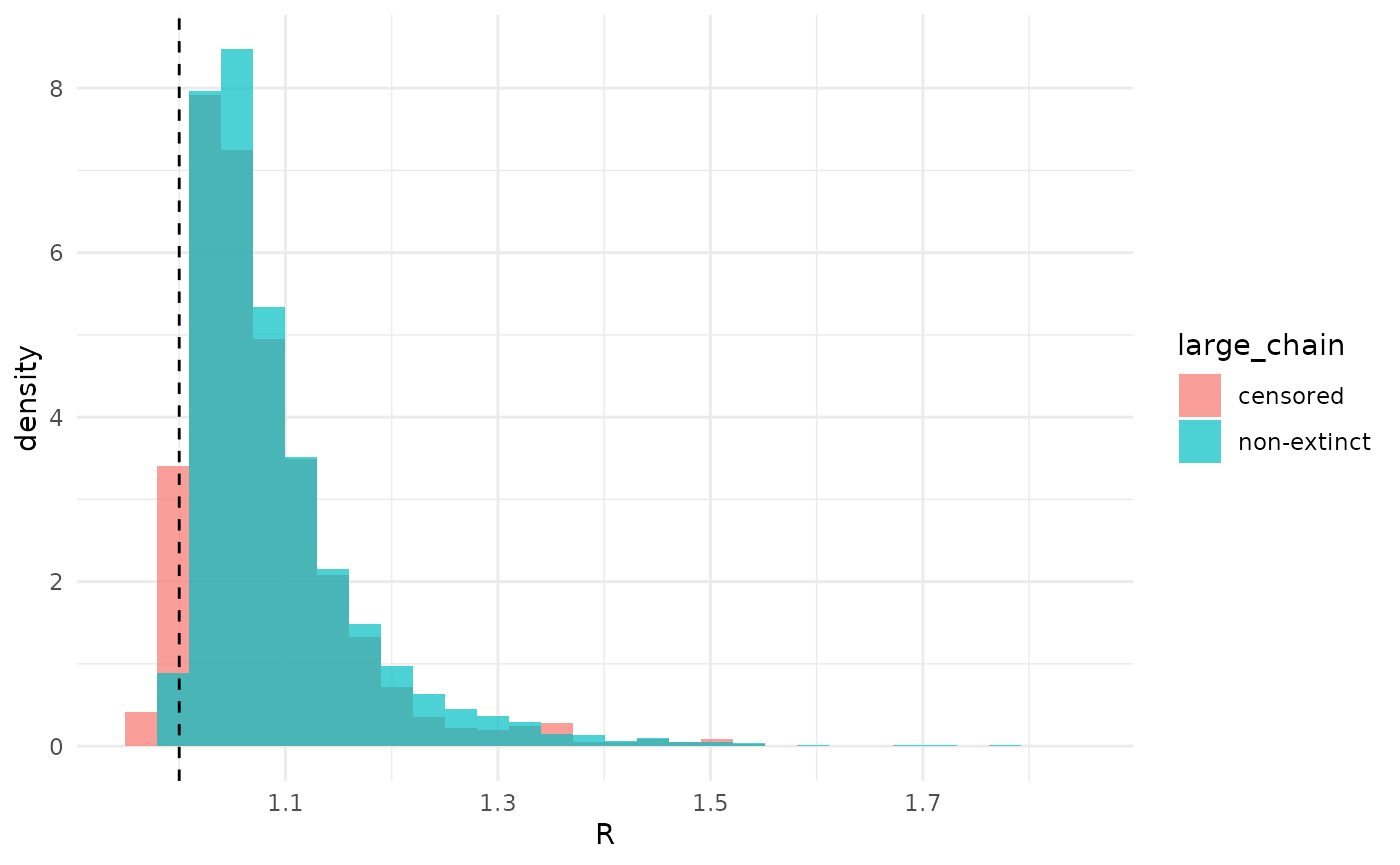

The overall similarity of inference suggests that, in some sense, the model “prefers” to consider the chain non-extinct even if we did not say it was such. Recall that when $R \geq 1$ , a chain may or may not go extinct, while when $R < 1$ extinction is certain. So, for the part of the posterior where $R < 1$ the chain must be finite-but-large, while for the rest it could be either finite-but-large or non-extinct. We can compute both the probabilities of the chain being finite-but-large and/or non-extinct given $R$ and $k$ , and ask which is larger. We can marginalize this over the posterior distribution on $(R,k)$ and use the percent of the posterior where the probability that the chain is non-extinct is larger than that it is finite-but-large as a measure of this preference

We will need to use the PMF (dnbbp) and CDF (pnbbp) functions from nbbp. (Here we use 500 samples for illustrative purposes, but in general one should use the entire posterior.)

probs <- rstan::extract(fit_cen, pars = c("r_eff", "dispersion")) |>
  as.data.frame() |>
  head(500) |>
  mutate(
    ccdf = purrr::map2_dbl(
      r_eff, dispersion, function(r_eff, dispersion) {
        1 - pnbbp(5008, r_eff, dispersion)
      }
    )
  ) |>
  mutate(
    pr_non_extinct = purrr::map2_dbl(
      r_eff, dispersion, function(r_eff, dispersion) {
        dnbbp(Inf, r_eff, dispersion)
      }
    )
  ) |>
  mutate(
    pr_large = purrr::map2_dbl(
      ccdf, pr_non_extinct, function(ccdf, pr_non_extinct) {
        ccdf - pr_non_extinct
      }
    )
  )

The probability that the chain is non-extinct is larger in 90% of the posterior, confirming our intuition.

Estimates of $k$ are even more similar between the two analysis choices than $R$ .

k_df <- data.frame(
  k = c(
    unlist(rstan::extract(fit_inf, "dispersion")),
    unlist(rstan::extract(fit_cen, "dispersion"))
  ),
  large_chain = c(
    rep("non-extinct", 10000),
    rep("censored", 1200)
  )
)

k_df |>
  ggplot(aes(
    x = log(k),
    fill = large_chain,
    y = after_stat(density)
  )) +
  geom_histogram(position = "identity", alpha = 0.7) +
  theme_minimal() +
  xlab("log(k)")

## `stat_bin()` using `bins = 30`. Pick better value `binwidth`.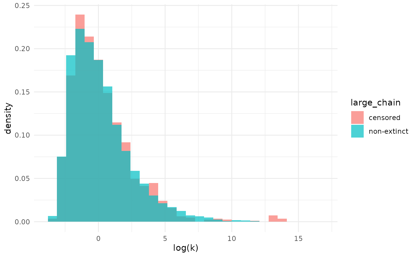

Note that while the analyses produced similar results here, that is not guaranteed to be the case in general. Differences are especially likely if the observed size of a non-extinct chain is not as large as it is here. Careful thought should be used to choose an analysis approach.

Missing cases

Another time where the observed chain size may not be the true chain size is when we have partially-observed chains That is, we have some, but not all, of the cases in any given chain. In nbbp, this can be handled using a binomial sampling model.

Mathematics of the likelihood

In this framework, a partially-observed chain has some observed size $c$ , an unobserved true size $u \geq c$ , and we assume that each observed case is independently sampled with probability $p$ . We compute the likelihood of the observed chain size by marginalizing out $u$ , yielding $\mathrm{Pr}(c \mid R, k, p) = \sum_{u = c}^\infty \mathrm{Pr}(c \mid u, p) \mathrm{Pr}(u \mid R, k)$ . The first term is the (binomial) probability of seeing $c$ of $u$ cases, the second is the NBBP probability of a chain having size $u$ . Unlike the censoring case, we cannot get clever with the law of total probability when computing this marginal. Instead, we use a sufficiently large $u_\mathrm{max}$ such that $\sum_{u = c}^{u_\mathrm{max}} \mathrm{Pr}(c \mid u, p) \mathrm{Pr}(u \mid R, k)$ is sufficiently close to the correct infinite sum. (Details on how the package chooses this value are available in the documentation for .get_partial_ub.)

Example

To examine the partially-observed scenario, we will work with simulated data. In our example, we will assume that all chains have a shared per-case sampling probability $p$ .

nchains <- 20

withr::with_seed(42, {
  true_chain_sizes <- rnbbp(nchains, r = 0.75, k = 0.25)
})
p <- 0.5

observed_chain_sizes <- true_chain_sizes
observed_chain_sizes <- rbinom(nchains, observed_chain_sizes, p)
print(paste0("Number of unobserved chains: ", sum(observed_chain_sizes > 0)))

## [1] "Number of unobserved chains: 11"

observed_chain_sizes <- observed_chain_sizes[observed_chain_sizes > 0]

print(paste0("Average true chain size: ", mean(true_chain_sizes)))

## [1] "Average true chain size: 3.4"

print(paste0("Average observed chain size: ", mean(observed_chain_sizes)))

## [1] "Average observed chain size: 3"

Our average observed chain size has decreased from 3.4 to 3. Why is the ratio of means 0.88 different from our per-case sampling probability of 0.5? Note that the presence of incomplete sampling also means we can lose entire chains. Here we’ve lost 9 out of the 20 we chose to simulate. These chains with no sampled cases are why the mean is different, and that we can’t see them is why we must condition the likelihood of partially-observed chains on sampling at least one case.

By default nbbp conditions all likelihoods on seeing at least one case in every chain. (When we have complete observations, this happens with probability 1 and can be ignored.) When inferring parameters from partially-observed chains, we need to tell nbbp what the sampling probabilities are. We do this on a per-chain basis, in case we have reason to believe that some have better or worse sampling than others. And as this parameter is not identifiable, we do not infer it but simply tell nbbp what it is. In real life, when we do not know, we can always perform analyses under a range of plausible values.

partial_geq <- observed_chain_sizes

partial_probs <- rep(p, length(observed_chain_sizes))

fit_incomplete <- fit_nbbp_homogenous_bayes(
  all_outbreaks = observed_chain_sizes,
  partial_geq = partial_geq,
  partial_probs = partial_probs,
  seed = 42
)

As always, first we inspect the MCMC, in this case finding it worked well.

rstan::check_hmc_diagnostics(fit_incomplete)

## 
## Divergences:

## 0 of 10000 iterations ended with a divergence.

## 
## Tree depth:

## 0 of 10000 iterations saturated the maximum tree depth of 10.

## 
## Energy:

## E-BFMI indicated no pathological behavior.

rstan::summary(fit_incomplete)$summary[, c("n_eff", "Rhat")]

##                        n_eff     Rhat
## r_eff               3421.015 1.000394
## inv_sqrt_dispersion 4309.687 1.001195
## dispersion          4667.817 1.000394
## exn_prob            3948.245 1.001210
## p_0                 4436.066 1.000665
## lp__                2187.246 1.002622

Now we can look at what we estimated.

fit_incomplete

## Inference for Stan model: nbbp_homogenous.
## 4 chains, each with iter=5000; warmup=2500; thin=1; 
## post-warmup draws per chain=2500, total post-warmup draws=10000.
## 
##                        mean se_mean        sd   2.5%    25%    50%    75%
## r_eff                  0.77    0.00      0.14   0.51   0.67   0.76   0.85
## inv_sqrt_dispersion    0.78    0.01      0.60   0.03   0.31   0.65   1.12
## dispersion          5619.44 4021.49 274753.89   0.20   0.80   2.37  10.20
## exn_prob               1.00    0.00      0.02   0.94   1.00   1.00   1.00
## p_0                    0.54    0.00      0.09   0.40   0.48   0.53   0.60
## lp__                 -25.53    0.02      1.10 -28.46 -25.98 -25.18 -24.75
##                       97.5% n_eff Rhat
## r_eff                  1.07  3421    1
## inv_sqrt_dispersion    2.21  4310    1
## dispersion          1253.31  4668    1
## exn_prob               1.00  3948    1
## p_0                    0.75  4436    1
## lp__                 -24.44  2187    1
## 
## Samples were drawn using NUTS(diag_e) at Fri Feb 27 20:05:01 2026.
## For each parameter, n_eff is a crude measure of effective sample size,
## and Rhat is the potential scale reduction factor on split chains (at 
## convergence, Rhat=1).

We can see that we estimated both $R$ and $k$ relatively well. Missing cases don’t have to be bad for inference, as long as we can appropriately accommodate them. Unfortunately, in the real world, matters can easily get more complex. No real observation process is as straightforward as the model, nor in general will we be sure about how what fraction of cases we have actually observed. Nevertheless, if we have a decent idea of what we might be missing (or a range of plausible values), and the binomial sampling model is not too badly misspecified, all is not lost.