Default priors

A Gamma prior is placed on $R$, and a HalfNormal on $1 / \sqrt{k}$. The user may specify hyperparameters of the Gamma distribution (its shape and rate) and the HalfNormal (its scale parameter). Samples from the default prior are available in the package data object prior_predictive (created by this script), which we will use to visualize the priors.

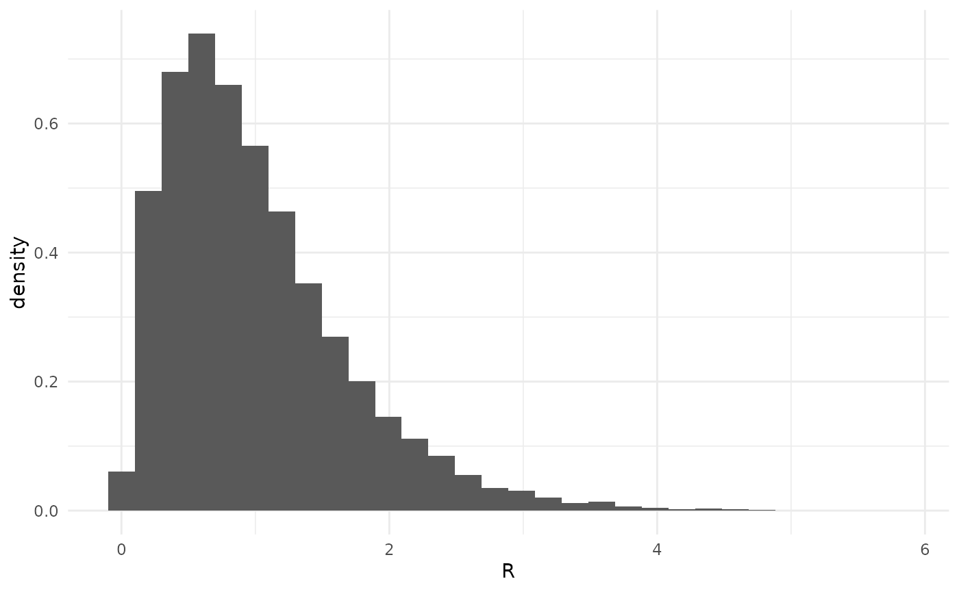
Default prior on $R$

The parameter $R$ is the average number of infections caused by one infected individual (that is, it is the reproduction number).

The default prior on $R$ is Gamma(shape = 2.183089, rate = 2.183089). This has a mean of 1 and stipulates that $R$ is most likely between 1/2 and 2 (with 66.67% of prior mass in this region). The choice of mean 1 serves to provide some prior regularization (pull) towards 1. In regimes where $R$ is small, this should make estimation somewhat conservative, erring on the side of larger $R$. The tradeoff is that in regimes where $R$ is large, we can under-estimate $R$. (For simulation-based testing of such performance, see the vignettes “Simulation-based testing” and “Simulation-based calibration.”)

Some might wonder why the prior on $R$ is not more informative, while others might wonder why it is not less informative. Broadly, the prior is intended to be slightly informative while simultaneously allowing the data to express themselves in regions of $R$ which may be encountered during expected usage of this package. Inference of $R$ from final size data under a negative binomial branching process model is strongly associated with the “stuttering chains” regime of non-sustained transmission. This is typically a subcritical ($R < 1$) regime, though with sufficient overdispersion (see below for the effect of $k$) is is possible in the supercritical regime.

Default prior on $k$

Note that the prior on $k$ is implicit (though we can still discuss it); the explicit prior is placed on $1 / \sqrt{k}$. The choice of a HalfNormal on $1 / \sqrt{k}$ follows best-practices for a “weakly” informative prior on the NegativeBinomial over-dispersion parameter.

The parameter $k$ controls the dispersion of the offspring distribution, as well as the final size distribution, and plays a strong role in the probability of extinction of a chain. When $k$ is large, there is less dispersion relative to the mean, and in the limit of $k \to \infty$, the NegativeBinomial approaches the Poisson. At $k = 1$, the NegativeBinomial coincides with the Geometric distribution. When $k$ is small, the variance of the offspring distribution gets larger, increasing the variance of the chain size distribution. This increase in variance also increases the probability that an individual has no offspring, increasing the extinction probability. In the limit as $k \to 0$, all chains die out after the index case and there is no information about $R$ whatsoever.

Since both $R$ and $k$ affect the extinction probability, our inference of one affects our inference of the other. Did the observed chains go extinct because most infections cause, on average, few new infections, or because many infections cause none at all, while others cause many? The prior pulls towards larger $k$, which, handwavily, means the model should prefer to answer this question in terms of the mean.

The default prior has a median $k$ of 1, placing 50% of the prior mass in both the strongly-overdispersed $k < 1$ regime and the less-overdispersed $k \geq 1$ regime.

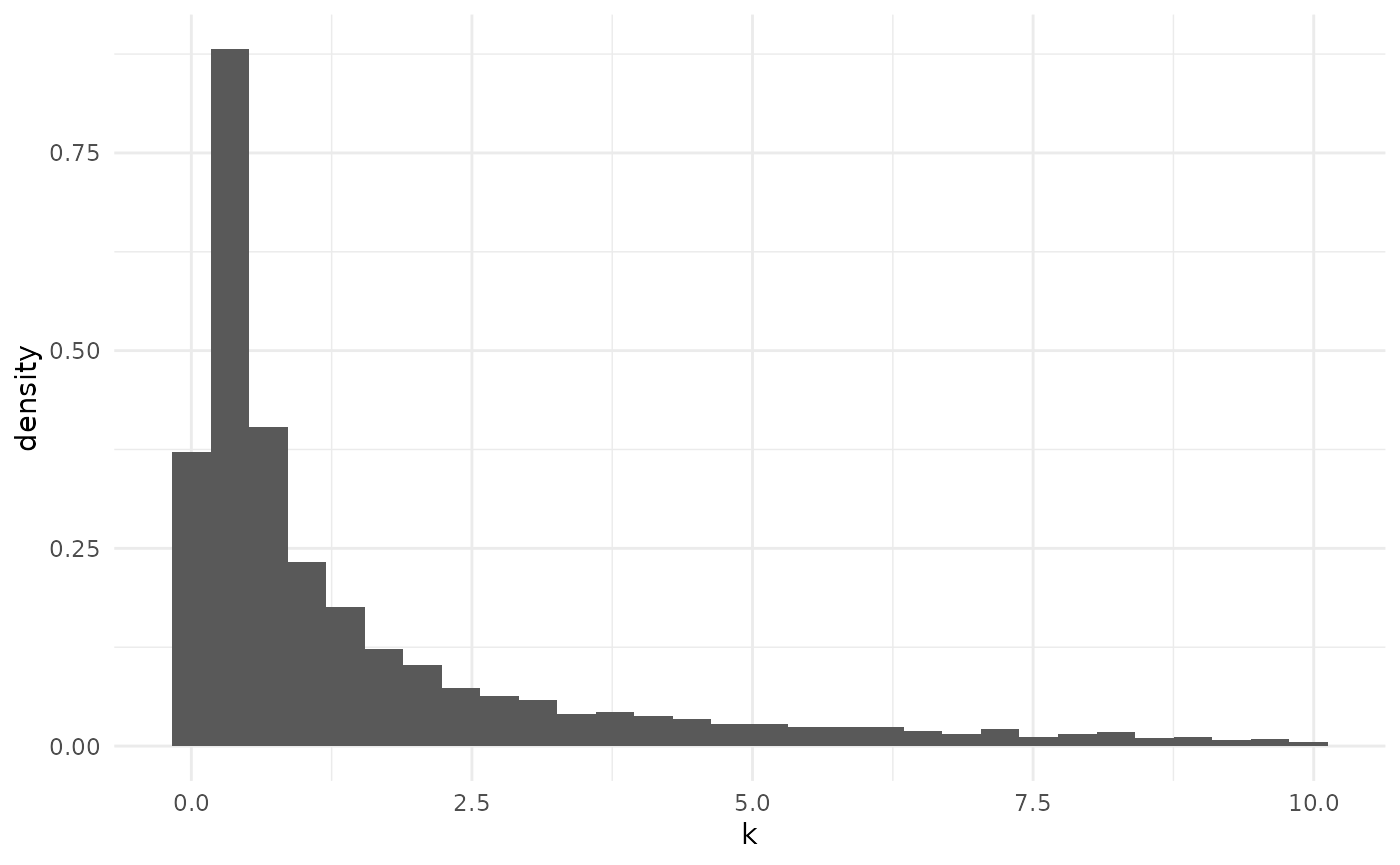
The (implicit) default prior on $k$ has heavy tails, reflecting the prior’s pull towards the Poisson regime of $k \to \infty$. Truncating to $k \leq 10$ for visualization purposes, the (conditional implicit) prior is

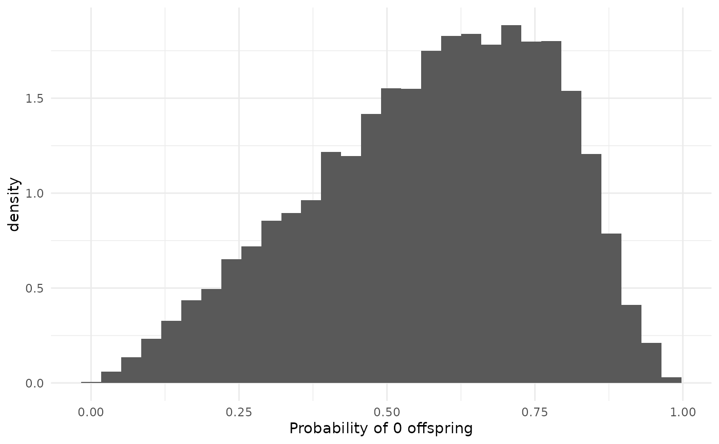
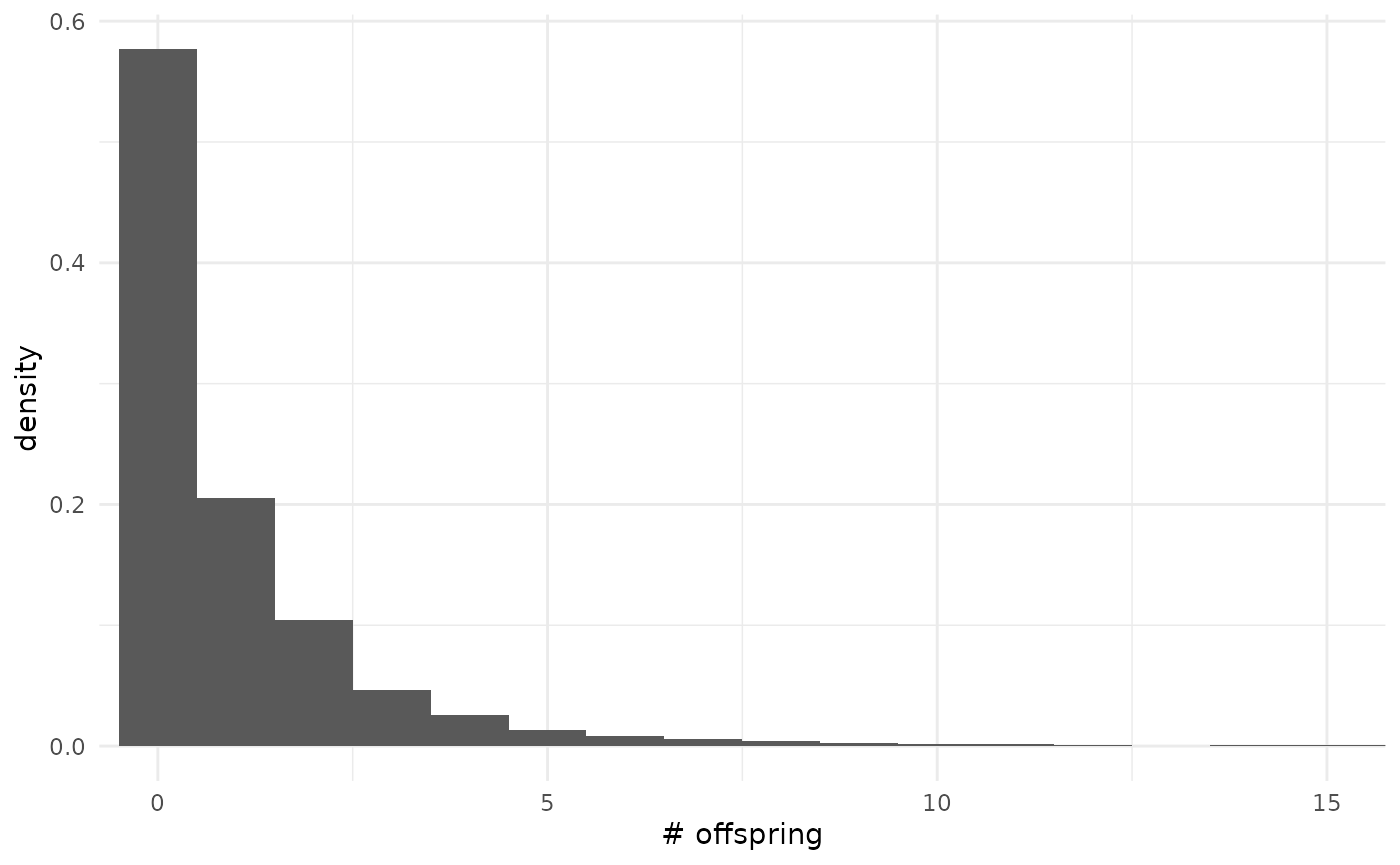
Default prior predictive offspring distribution

Conditioned on $R$ and $k$, the offspring distribution is negative binomial. By marginalizing this conditional distribution across the priors on $R$ and $k$, we obtain the prior predictive offspring distribution.

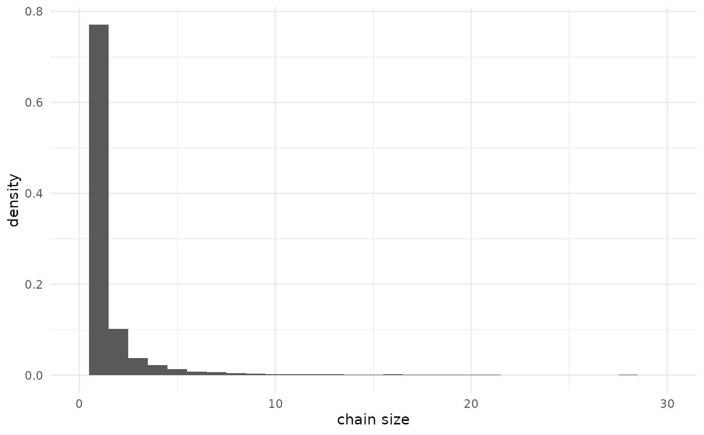
Default prior predictive chain size distribution

The prior predictive distribution on chain sizes has two components. There is a 14% chance of a non-extinct (infinite) chain (see the vignette “Advanced data” for more on this). Conditional on extinction (finite size), there are long tails, with a 14% chance of a chain size above 100. Focusing in on chains of 100 or fewer for visualization, the (marginal with respect to $R$ and $k$, conditional with respect to the chain size) prior distribution is:

Implicit default prior on p_0

The samples from the prior predictive offspring distribution gives us a marginal summary of the probability that an infection produces no offspring. But we can also look at its implied prior distribution, as it is a function of $R$ and $k$.