Implementation details

Conditioning and multimodality of the likelihood surface

As can be seen in the vignette “nbbp,” the likelihood surface sometimes has a mode at 0. It can also be multimodal when conditioning is applied.

Conditioning on observation sizes

In particular, multimodality can be induced when conditioning on observing chains of at least some size. An example of this can be seen using the pneumonic plague data considered in “Advanced data” where the likelihood must be conditioned on observing at least two cases to match the data-collection process.

library(nbbp)
library(ggplot2)
data(pneumonic_plague)

pneumonic_plague[4] <- Inf

lnl_surface <- compute_likelihood_surface(
  pneumonic_plague,
  condition_geq = rep(2, 19),
  r_grid = seq(1.0, 1.35, length.out = 100),
  k_grid = exp(seq(log(0.01), log(9999), length.out = 100))
)

lnl_surface |>
  dplyr::mutate(
    log_dens = ifelse(log_dens >= max(log_dens) - 1, log_dens, NA)
  ) |>
  ggplot(ggplot2::aes(x = r, y = k, fill = log_dens)) +
  theme_minimal() +
  geom_tile() +
  scale_y_continuous(transform = "log") +
  scale_fill_viridis_c(option = "magma")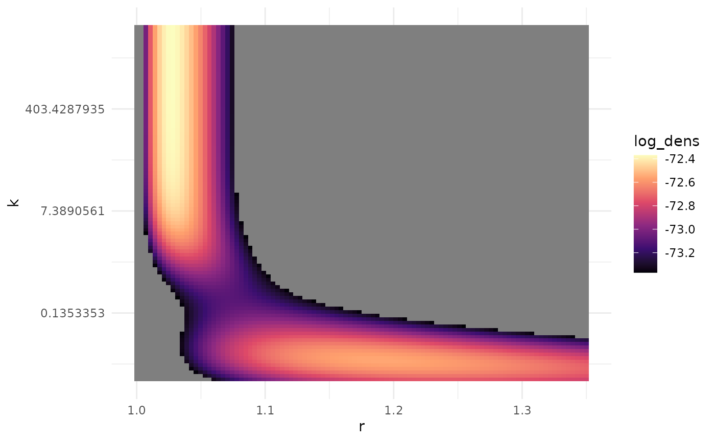

Inferring an unconstrained $R$

Some applications of the negative binomial branching process model have conditioned the likelihood on extinction to study the $R > 1$ case. In this way, it can be guaranteed that all chain sizes are finite, even when infinite chains are possible. However, Waxman and Nouvellet (2019) show that when conditioning there are two indistinguishable modes, one with $R > 1$ and one with $R < 1$. For this reason, we treat non-extinct chains separately in both stan code for inference and R code for simulation. In inference, a non-finite chain provides guarantees that $R > 1$, this is the necessary condition for a negative binomial branching process to never go extinct. Therefore, the presence or absence of such chains is itself informative (see the vignette “Advanced data” for an application). In simulation, this means that when $R > 1$, some samples may be Inf, indicating a non-extinct chain.

Mathematically, we partition the model outcomes into finite and infinite chains. That is, a chain either goes extinct (has finite size) or doesn’t, and this happens according to the extinction probability $\text{Pr}(\mathcal{E} \mid R, k)$. Formally, the possible chain sizes are $c \in \{0, 1, \dots\} \cup \infty$. We can write the likelihood for one chain size $c$ as $$\begin{equation} \text{Pr}(c \mid R, k) = \mathbb{I}(c \in \{0, 1, \dots\}) \left[ \text{Pr}(c \mid R, k, \mathcal{E}) \text{Pr}(\mathcal{E} \mid R, k) \right] + \mathbb{I}(c \in \{\infty\}) \left[ 1.0 - \text{Pr}(\mathcal{E} \mid R, k) \right] \end{equation}$$ where the chain size which can take finite values $c = 0, 1, \dots$ as well as the value “$c = \infty$”, $\mathbb{I}$ is the indicator function, and $\mathcal{E}$ ($\mathcal{E}^{\text{C}}$) is the event that the chain goes (does not go) extinct. For conditionally finite chains, we can write $$\begin{equation} \text{Pr}(c \mid R, k, \mathcal{E}) = {\text{Pr}(c, \mathcal{E} \mid R, k) \over \text{Pr}(\mathcal{E} \mid R, k)} = {\text{Pr}(c \mid R, k) \over \text{Pr}(\mathcal{E} \mid R, k)}. \end{equation}$$ Using this expression reduces the likelihood of chain size $c$ to $$\begin{equation} \text{Pr}(c \mid R, k) = \mathbb{I}(c \in \{0, 1, \dots\} ) \left[\text{Pr}(c \mid R, k) \right] + \mathbb{I}(c \in \{\infty\}) \left[ 1.0 - \text{Pr}(\mathcal{E} \mid R, k) \right]. \end{equation}$$

Numerical approximations

Probability of extinction

Except for very specific values of $k$, the extinction probability is not available in closed form. In stan, we use Newton’s method to obtain a numerical solution when it is needed.

CDF

While the PMF for the chain-size distribution is available in closed form, there is no closed form solution for the CDF.

Compromises for efficiency

For efficiency, when drawing random chain sizes the package uses base::sample() on a pre-computed, truncated, set of values. This enables rapidly sampling many realizations for a pair of $R, k$ values. Truncation is hard-coded at 1,000,000 which in practice appears to cover at least 99.999% of the probability mass. The most mass is unaccounted for when $R = 1$ and $k \to 0$.

Censoring

When brute-force computing the CDF (by summing the PMF), sometimes it evaluates to numbers slightly greater than 1. In practice, this appears to happen exclusively for $R < 1$ and the maximum seems to be less than $1 + 10^{-12}$. This is noticeable when censoring observations, where for chain size $c$ we need $\text{Pr}(C >= c) = 1 - \text{CDF}(c - 1)$. When the CDF exceeds one, this is negative and MCMC cannot appropriately explore the $R < 1$ region. To avoid these issues, the stan model code checks that the CDF does not exceed 1 over the range it needs to be evaluated. If it ever exceeds 1, we rescale so that the maximum CDF is 1.0 - machine_precision().

Approaches for confidence intervals

While profiling of the likelihood is a common approach for generating confidence intervals for the negative binomial branching process model, we found that univariate profiling produced CIs with poor coverage properties for much of parameter space. Except near $R = 1$, the parametric bootstrap (repeatedly simulating data from the fit model and fitting to the simulated data) provides notably better coverage. Thus the default method for CI generation is a hybrid approach, using the parametric bootstrap unless the profile-based interval would be superior. This is implemented by checking whether the profiling confidence interval crosses 1, in which case it is used, or not, in which case parametric bootstrapping is used.