Running MIRA-CLI with Illumina Data
![]()
This documentation assumes you have the MIRA Docker container already running. If not, please start with PC Getting Started, MAC Getting Started and MIRA install instructions.
Fill out Samplesheet
You will need to create your samplesheet.csv before running MIRA-CLI.
The format within the samplesheet should be as follows:
- Sample names should only be numbers, letters, dashes, and underscores (“-” or “_“). Do not use any other characters such as “/”.
- Select your
Sample Type. Most of your sample’s are test samples, so each row defaults totest, but select- controlor+ controlfor your negative and positive controls respectively. - Save your samplesheet with changes as a csv
Stage your demultiplexed data
- In your “MIRA_NGS” folder, make a folder for your run. It is very helpful to name your runs with a consistent naming system, such as “YEAR-MONTH-DATE-FLOWCELL_ID”, ie. 2022-11-13-ABC1234.
DO NOT PUT SPACES OR SLASHES IN YOU RUN FOLDER NAMES!
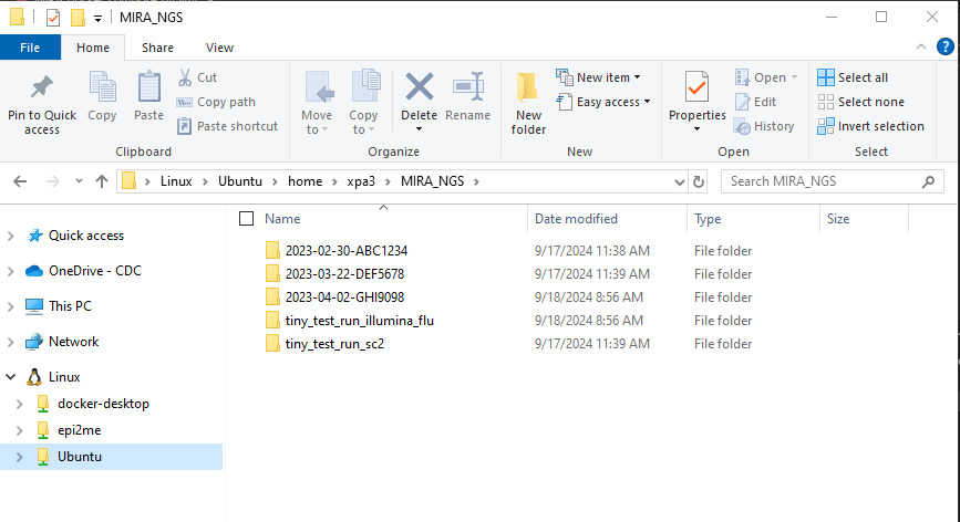
- Copy the run’s demultiplexed fastqs into the RUN-FOLDER.
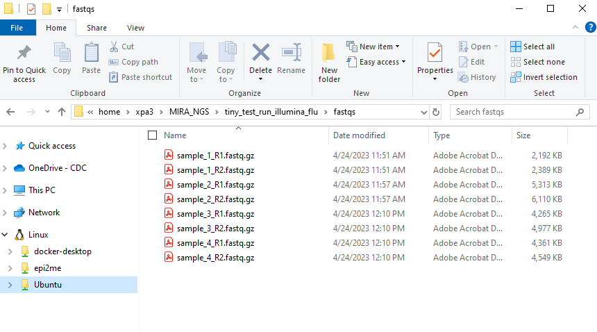
- Create another folder inside your RUN-FOLDER called “fastqs” and copy the folder containing demultiplexed, gunzipped fastqs into this newly created fastqs folder so that the folder structure is MIRA_NGS/RUN-FOLDER/fastqs/sample_R[1 and 2].fastq.gz There will be two fastq files per sample.
This screenshot shows WSL distro “Ubuntu-20.04” but many
users just see “Ubuntu”. This can vary, particularly if you happen to
have multiple Ubuntu versions installed. If you have multiple Ubuntu
distributions installed, move the fastqs to whichever “Ubuntu” contains
MIRA_NGS within home>USERNAME>MIRA-NF
Run Genome Assembly with MIRA-CLI
Start the MIRA container
- If MIRA is running, you should see it listed when you run
docker ps
Move to the MIRA_NGS folder
To run MIRA in the command line you will execute this command:
docker exec -w /data mira MIRA.sh -s run_folder/samplesheet.csv -r run_folder -e experiment_type -p primer_schema (optional)Within the command you will change these flags to match your data:
- s - your_run_folder/samplesheet.csv
- r - your_run_folder
- e - Flu-Illumina, SC2-Whole-Genome-Illumina, RSV-Illumina
- p - SC2 options: articv3, articv4, articv4.1, articv5.3.2, qiagen, swift, swift_211206 or RSV options: RSV_CDC_8amplicon_230901, dong_et_al
There will be a lot of standard error messages that print while MIRA
is running. It will look like the picture below: 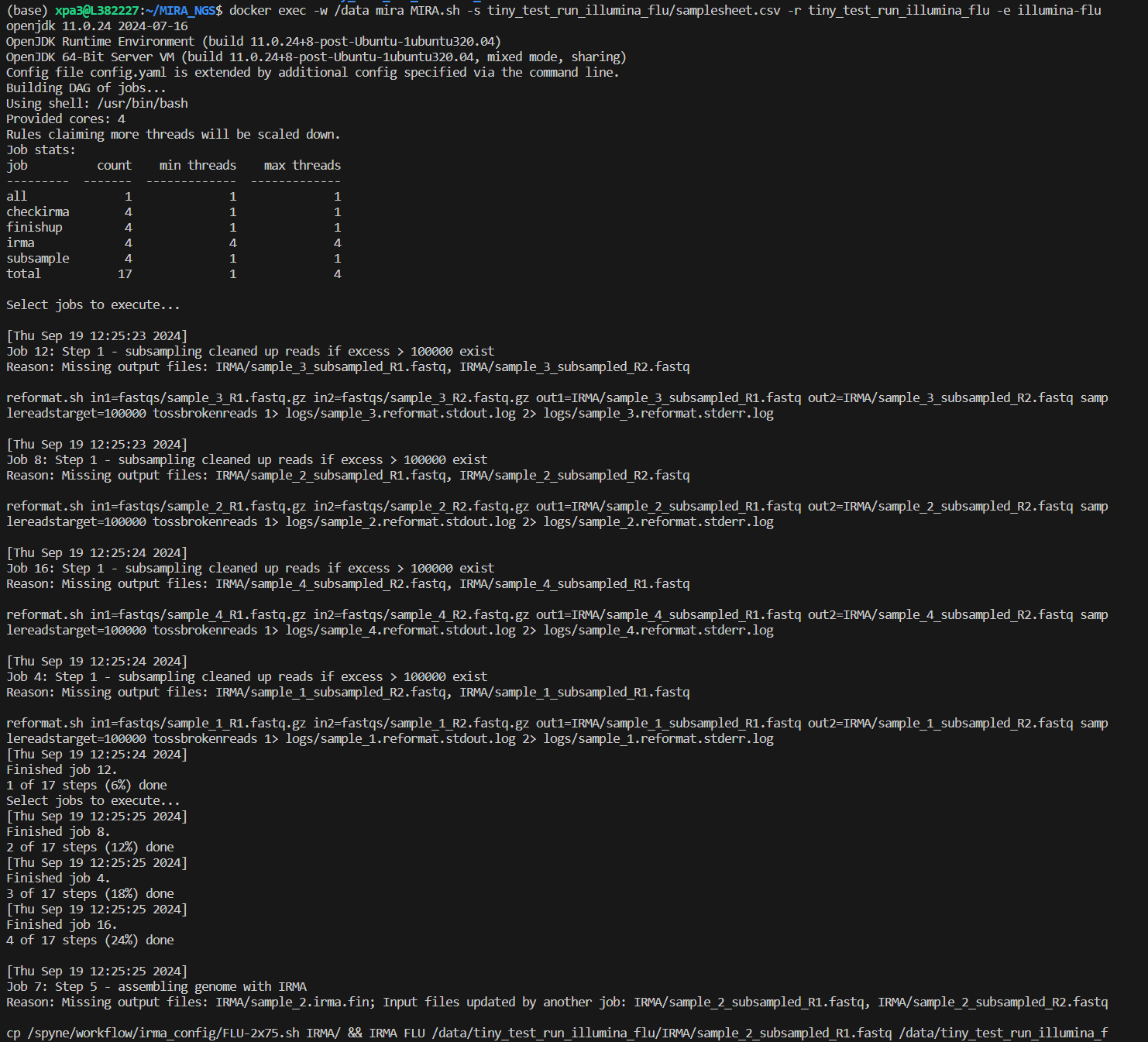
MIRA-CLI Ouputs
After MIRA has successfully completed its analysis, the following outputs should be within the run folder regardless of the experiment type indicated:
 Note that files are
named with the name given to the run folder
Note that files are
named with the name given to the run folder
If you open the MIRA-summary HTML it will look very similar to the summary provided in the GUI. It contains many of the same summary figures. To view the outputs in the MIRA GUI see below
For all of the download links to work within the MIRA-summary HTML, it must have the other files that were created with it present in the same directory (e.g. the amended_consensus.fasta, minorvariants.xlsx, etc.).
Key differences between the summary html and the summary in the GUI:
- There are only individual coverage files present for download.
- The minor variants and indels tables are only available for download.
FASTA files:
- amended_consensus.fasta - Nucleotide sequences that passed QC
- failed_amended_consensus.fasta - Nucleotide sequences that did not pass QC
- amino_acid_consensus.fasta - Amino acid sequences that passed QC
- failed_amino_acid_consensus.fasta - Amino acid sequences that did not pass QC
Excel files:
- aavars.xlsx - The amino acids variant table. If you see special characters see below
- minorvariants.xlsx - The single nucleotide variants (minor SNVs) table
- minorindels.xlsx - The minor insertions and deletions table
- summary.xlsx - This summaries the coverage stats from the IRMA assemblies, QC information determined by IRMA and read count information.
There will also be individual coverage HTML files for each sample input.
The IRMA folder contains the IRMA assemblies and full output with each sample getting its own folder. There will also be a folder within the IRMA folder label ‘dais_results’ that contains the inputs and output from DAIS Ribsome. The subsampled (and trimmed if applicable) fastq files will also be stored within this folder. We summarize all the information found in these folder in the reports listed above.
The dash-json folder contains all of the json files from which the GUI builds it’s figures. We recommend that you keep these files as they contain the key results from your analysis. See below for more information about the file archival process
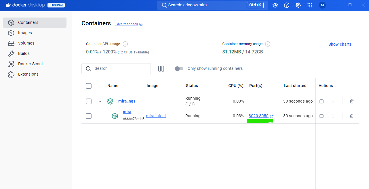
View Results in MIRA-GUI
-
Open MIRA by clicking the blue link “8020:8050”. This will open MIRA into your default internet browser. You can “bookmark” this site in your browser.
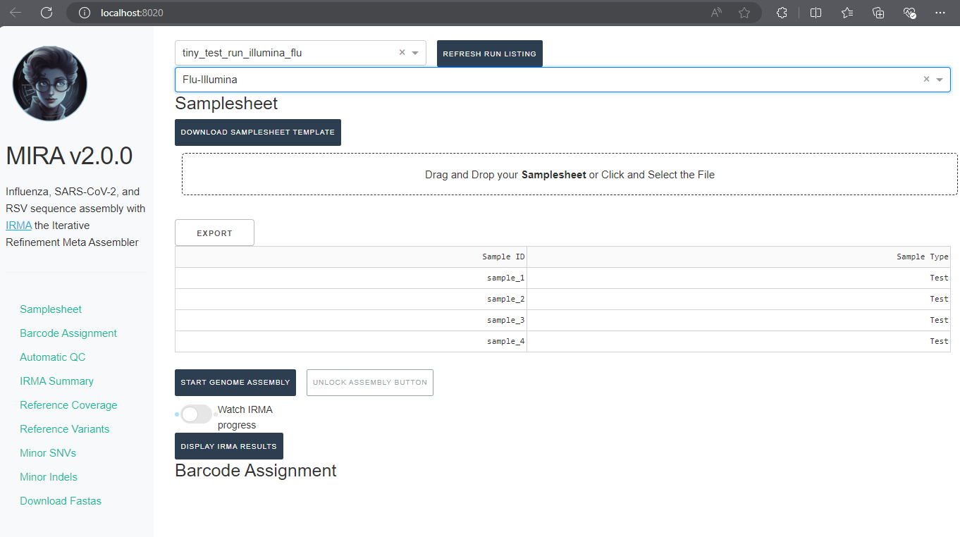
Select runs, data type, and enter sample information
-
Click the
REFRESH RUN LISTINGbutton and select your run from the dropdown box.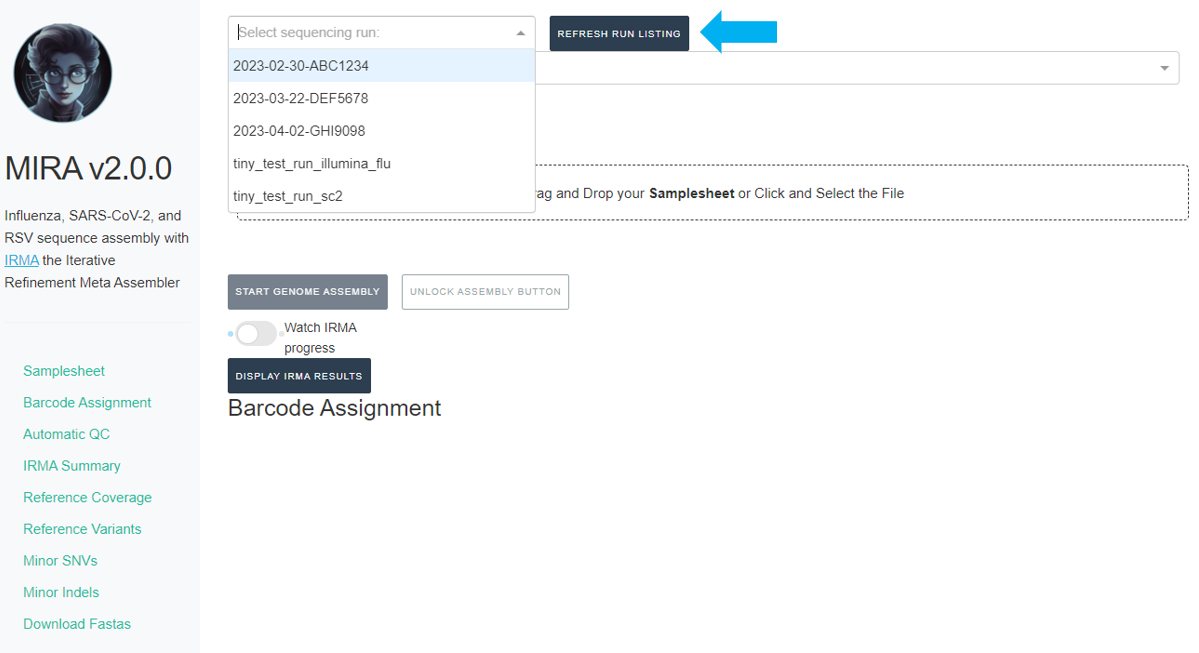
- Next, click the box that say “What kind of data is this” and select the data type you used for analysis
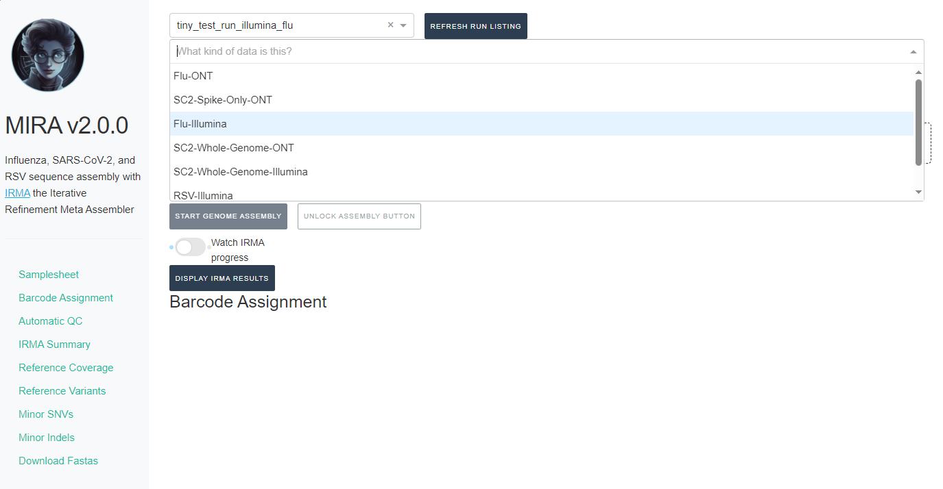
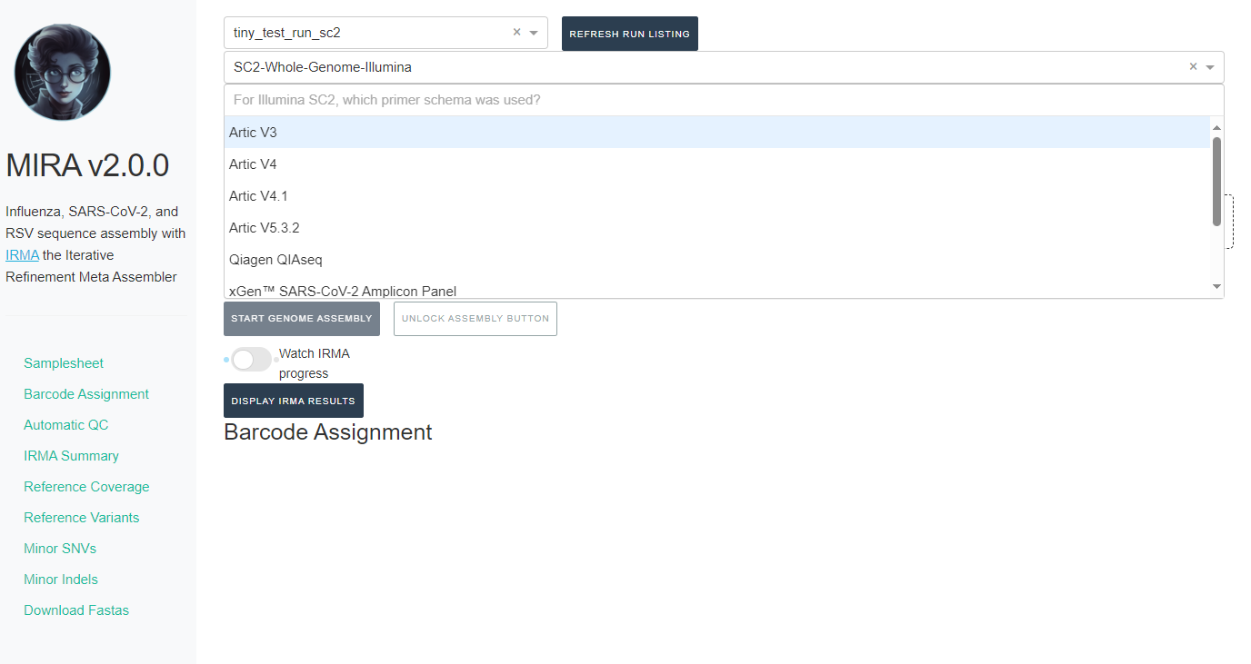
-
If you select SC2-Whole-Genome-Illumina or RSV-Illumina, a new box will appear for you to select your primer schema/amplicon approach
-
NOTE: MIRA SC2-Whole-Genome-Illumina and RSV-Illumina module’s
primer trimming steps have been tested and optimized for the primer
panels provided. We cannot guarantee perfect trimming for other
panels.
-
NOTE: MIRA SC2-Whole-Genome-Illumina and RSV-Illumina module’s
primer trimming steps have been tested and optimized for the primer
panels provided. We cannot guarantee perfect trimming for other
panels.
After filling out those fields you should see your samplesheet in the GUI.
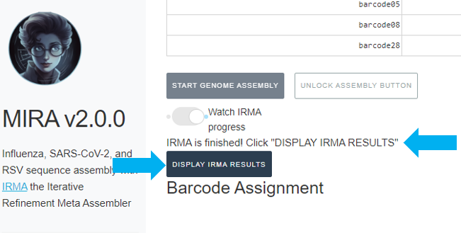
It will also say “IRMA is finished” and you can now click on “DISPLAY IRMA RESULTS”.
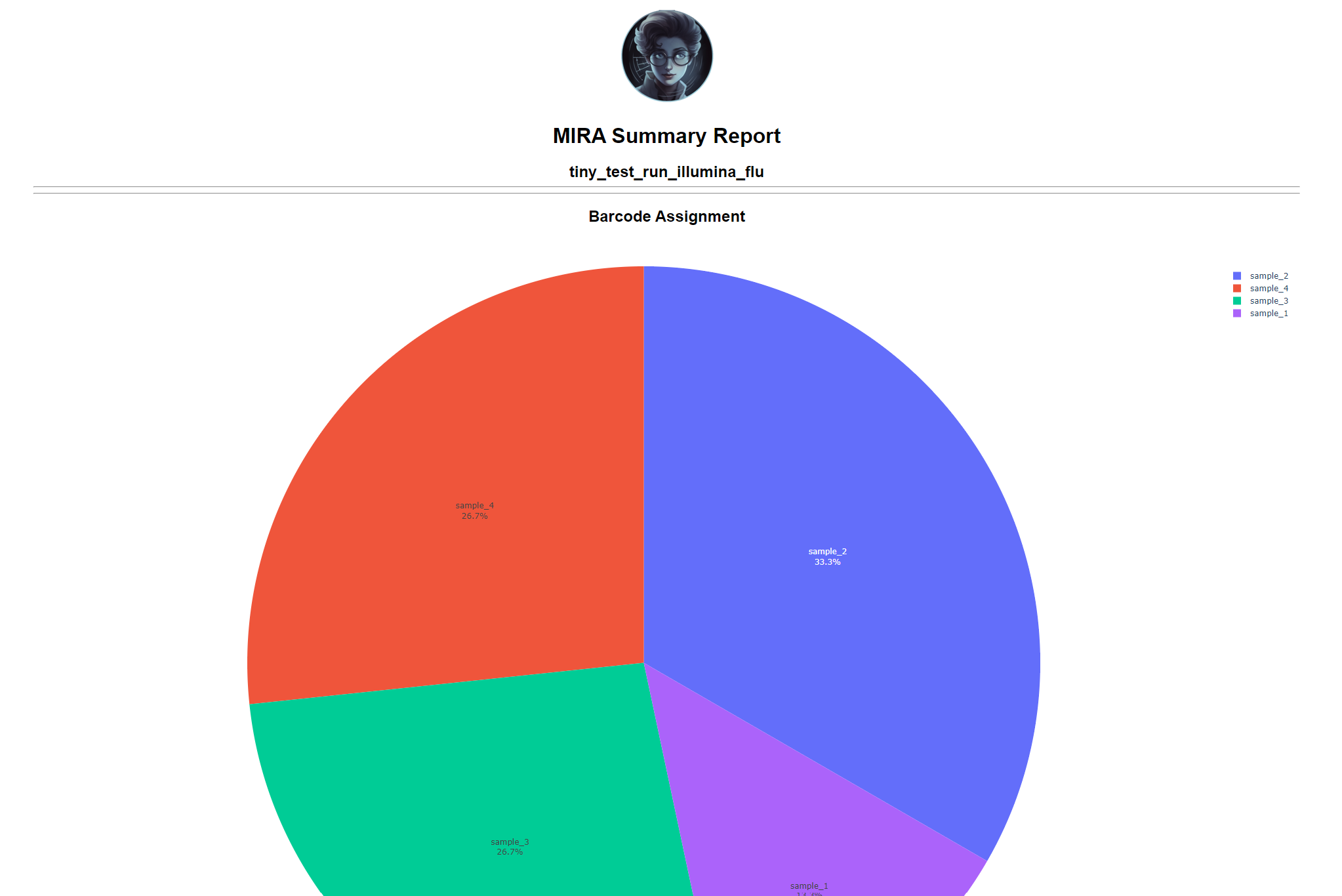
Review IRMA results
-
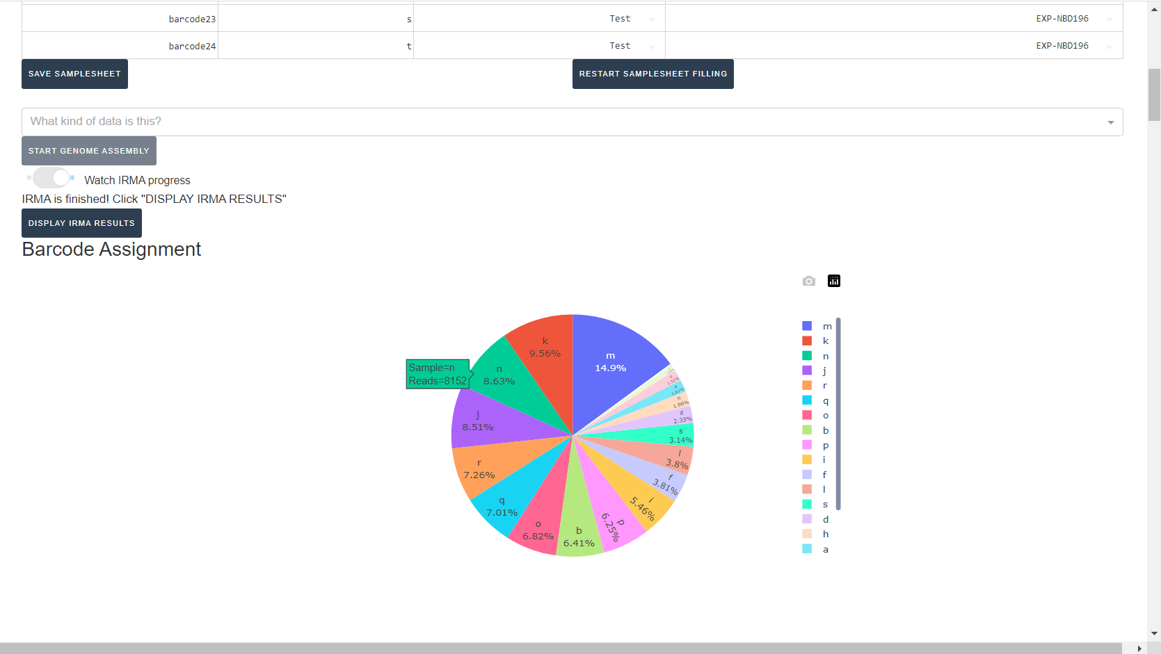
Review the distribution of reads assigned to each barcode. The ideal result would be a similar number of reads assigned to each test and positive control. However, it is ok to not have similar read numbers per sample. Samples with a low proportion of reads may indicate higher Ct of starting material or less performant PCR during library preparation. What is most important for sequencing assembly is raw count of reads and their quality.
-
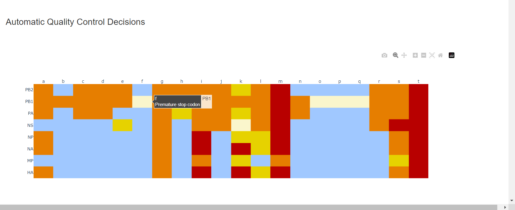
Review the “Automatic Quality Control Decisions” heatmap. In addition to IRMA’s built in quality control, MIRA requires a minimum median coverage of 100x, a minimum coverage of the reference length of 90%, and checks for minor variant counts indicative of contamination. See our QC standars page for all thresholds. These are marked in yellow to orange according to the number of these failure types. Samples that failed to generate any assembly are marked in red. In addition, premature stop codons are flagged in yellow. CDC does not submit sequences with premature stop codons, particularly in HA, NA or SARS-CoV-2 Spike. Outside of those genes, premature stop codons near the end of the gene may be ok for submission. Hover your mouse over the figure to see individual results.
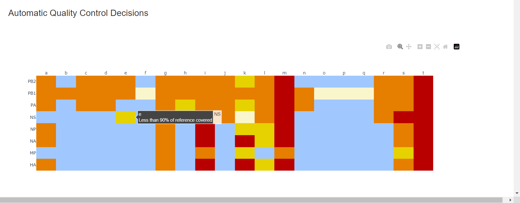
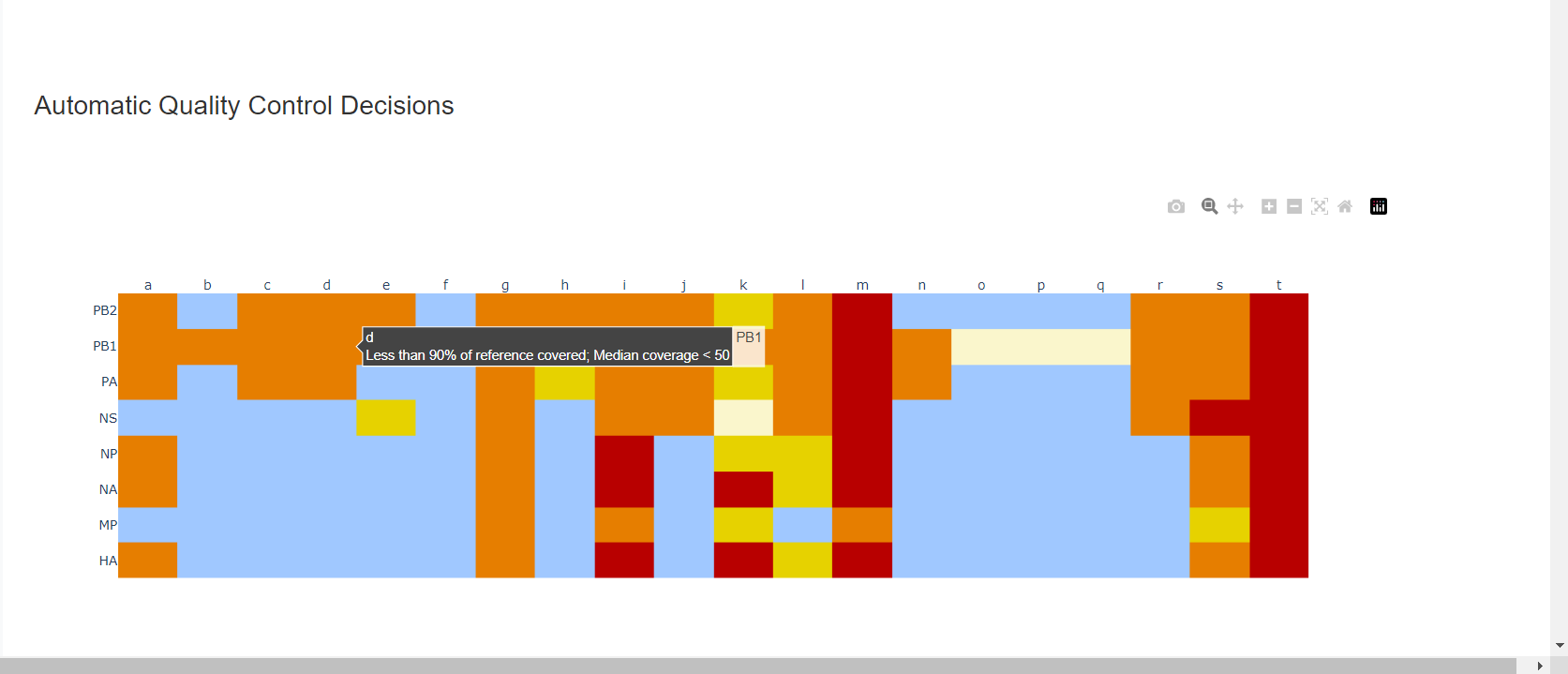
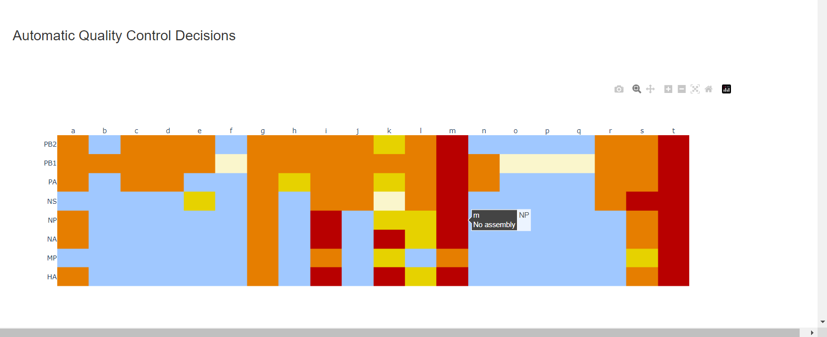
– – -
Review
MIRA Summary. This summarizes the above information, as well as detailed read assignment to specific referencs, in a table. Columns can be sorted and filtered, ie.>1000. ClickExportto save this as an Excel file.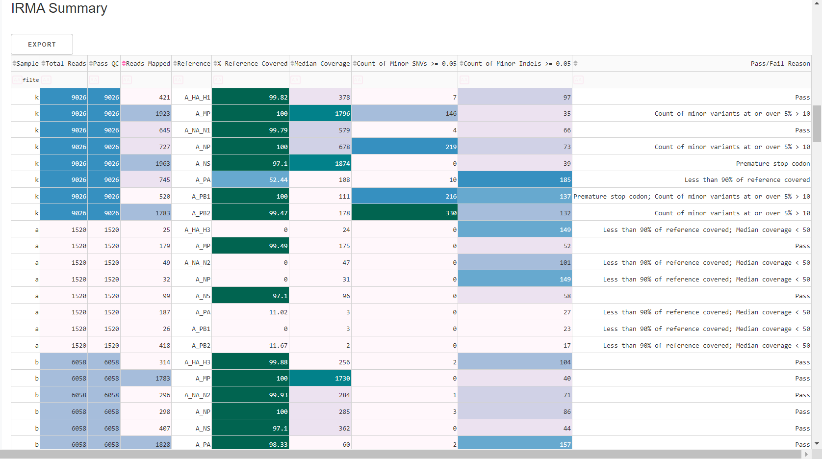
-
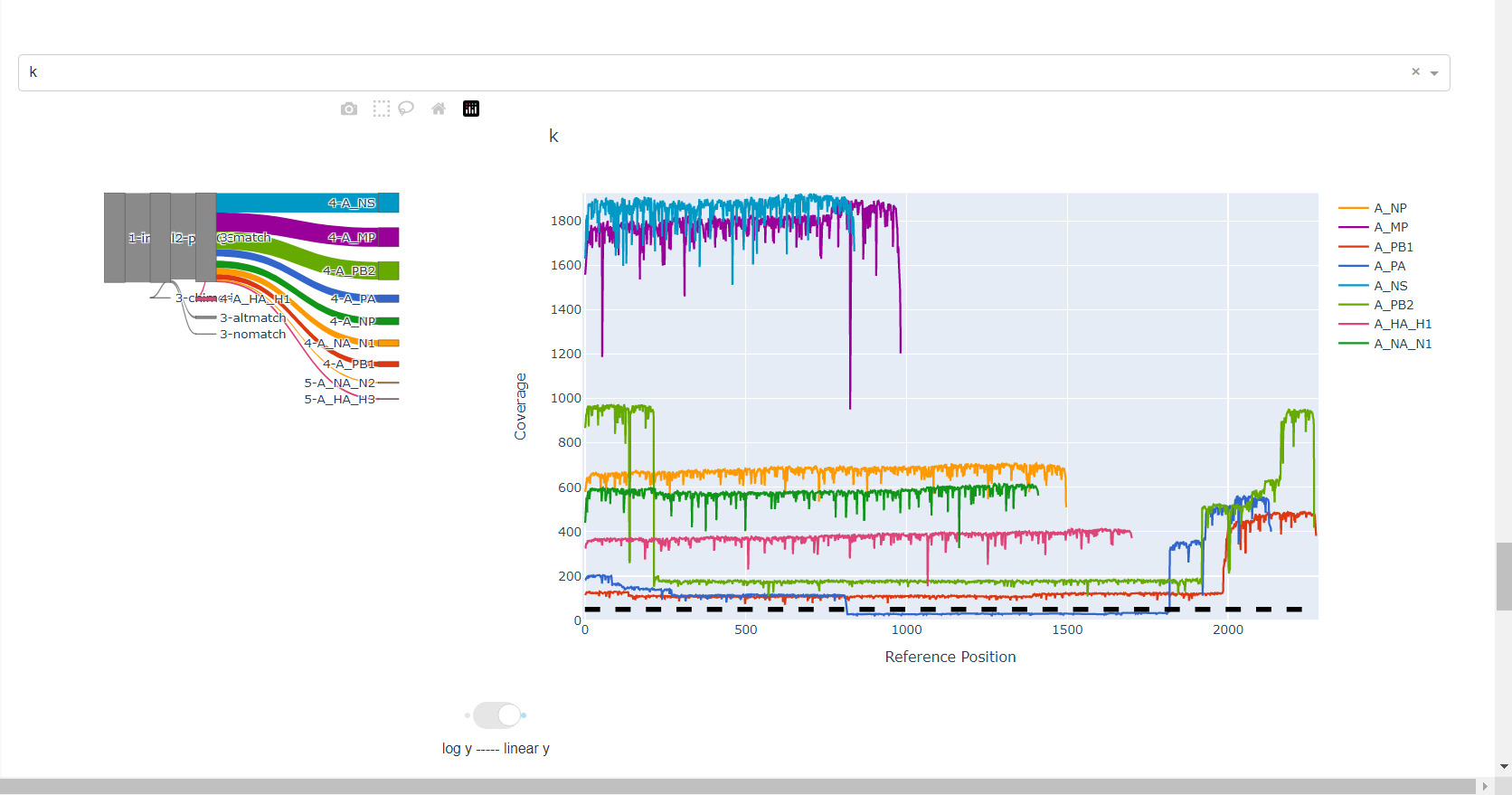
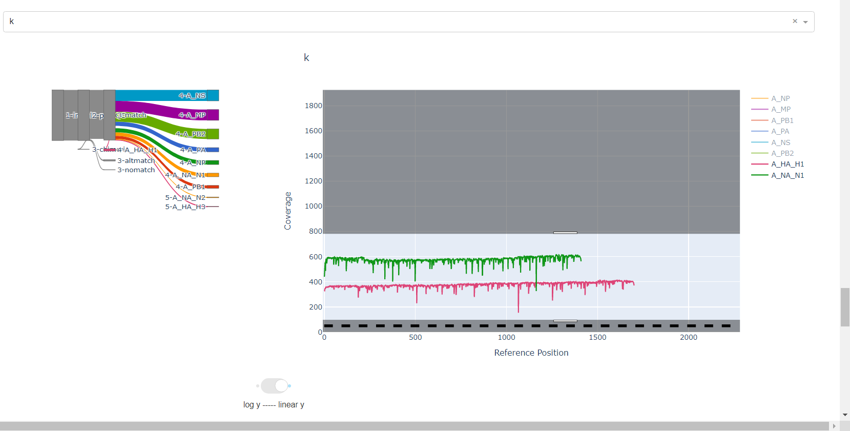
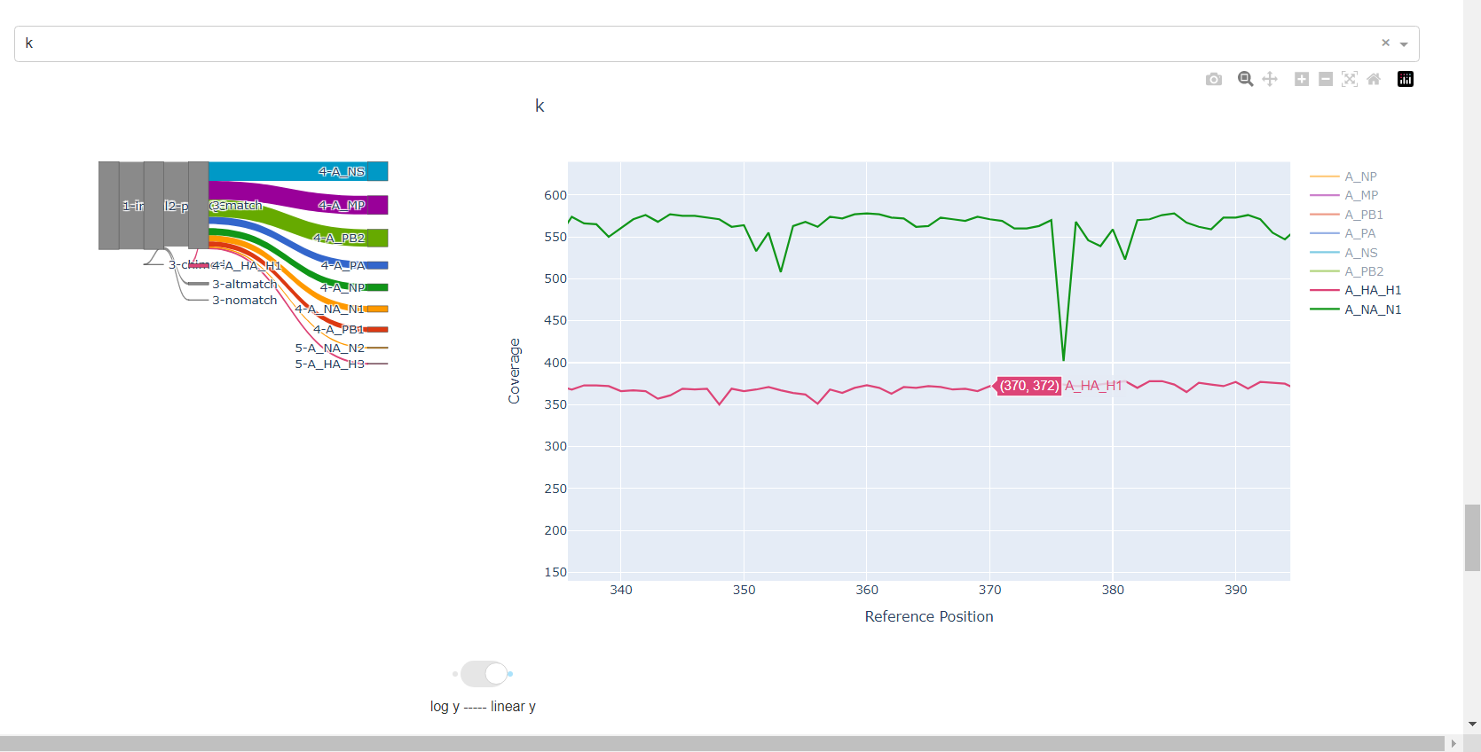
Review genome coverage depth. The heatmap summarizes the mean coverage per sample per gene. For all MIRA figures, you can click the gray buttons on the top right of the images. The camera icon will save the image. Clicking on a sample in the heatmap, or selecting one in the drop down menu will display two plots. On the left is a “sankey plot” that shows the number of reads assigned to the barcode, how many of those passed IRMA’s QC, and how many are assigned to each gene reference. The plot on the right shows the sample’s complete coverage per gene. Try toggling the
log y --- linear ybutton. In log space, you likely need to reset the view by clicking the gray button in the top right that looks like an X inside of a box. You can also try panning and zooming the plot.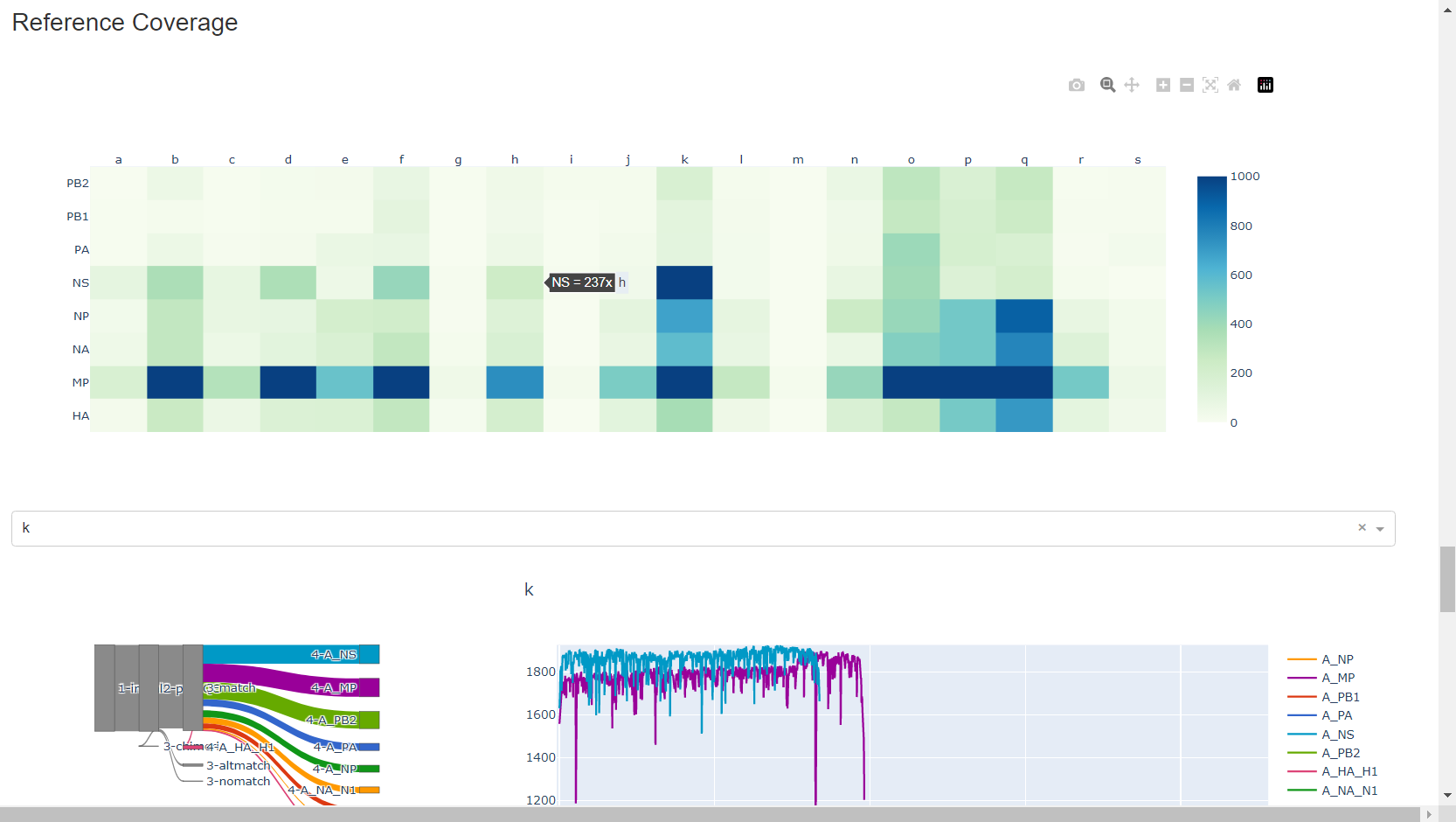
-
Inspect amino acid variants against popular reference sequences.
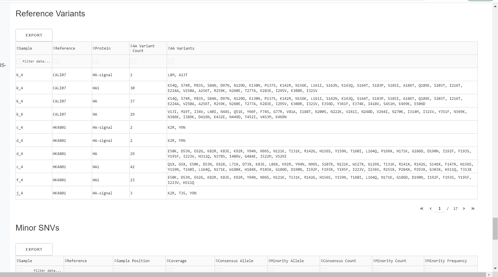
Here, you may see some mutations that do not match Amino Acid letters.
Special translated characters
Translation produces standard amino acid codes with the two non-standard exceptions (. and ~) listed below. The translation engine stops when it encounters a stop codon, but corrects itself to continue in-frame when a frameshift is encountered.
| Character | Interpretation |
|---|---|
| . | Missing alignment data |
| - | Gap in alignment (ex: deletion) |
| ~ | Partial codon (ex: frameshift) |
| X | Ambiguous codon translation |
-
Inspect minor variation at single nucleotides, insertions and deletions relative to the sample’s generated consensus sequence. These tables are for your own usage and not necessary to review in detail. They can be sorted and filtered and exported to excel sheets for further analyses.
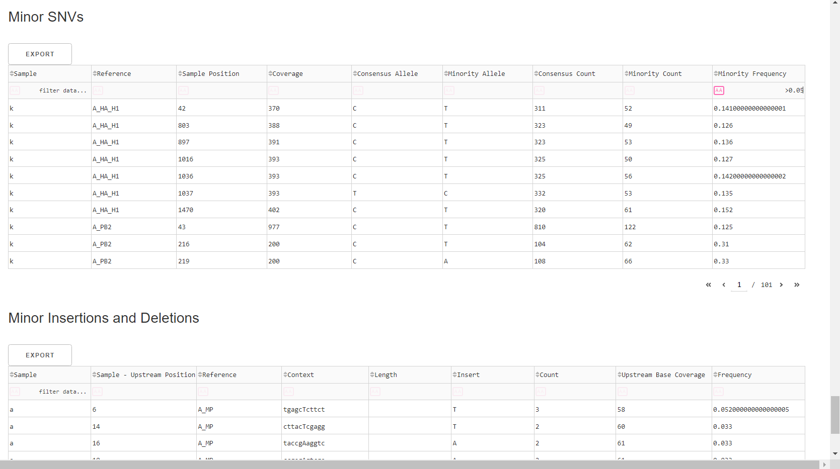
- Minor variants greater than 5% frequency are shown
- Indels greater than 20% frequency are shown
Save your sequences in a fasta file
-
Export IRMA’s amended consensus nucleotide sequences and amino acid fasta files. This includes only those passing MIRA’s QC criteria and are ready for submission to public databases!
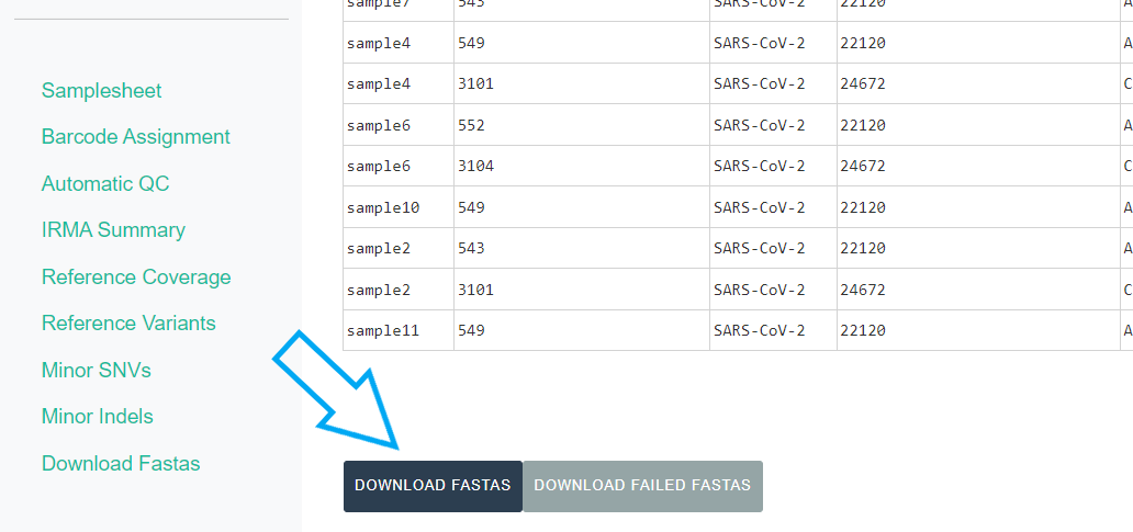
The
DOWNLOAD FASTASbutton will only return passing samples. To investigate failed sequences, click theDOWNLOAD FAILED FASTASbutton. Do not submit failed samples to public repositories!You can open and view these Amino Acid and Nucleotide fastas in any sequence viewing application

Archiving Files
Files that we recommend keeping:
- The original raw FASTQ files and the samplesheet.csv.
- All files within the dash-json folder.
- The amended consensus fasta files
You should keep any of the fasta files, excel files or html files described above that you believe will be useful to you.
Files that can be discarded:
- The IRMA folder and all of it’s contents.
- The logs folder and all of it’s contents.
- The .snakemake folder and all of it’s contents
- Any .fin files
Wow! You are doing such great work. Time to share your sequences with the world by uploading to GISAID and/or NCBI and to start analyzing your own data!
- GISAID: https://gisaid.org/
- Please indicate in your GISAID submission “MIRA” for the
assembly methodmetadata field
- Please indicate in your GISAID submission “MIRA” for the
- NCBI-Genbank: https://www.ncbi.nlm.nih.gov/genbank/
- NCBI-BLAST: https://blast.ncbi.nlm.nih.gov/Blast.cgi
- Nextclade: https://clades.nextstrain.org/