Fitting a basic renewal model

This tutorial shows the steps to build a simple renewal model featuring a latent infection process, a random walk \(\mathcal{R}(t)\) process, and an observation process for the reported infections.

We start by loading the needed components to build a basic renewal model:

import jax.numpy as jnp
import numpy as np
import numpyro
import numpyro.distributions as dist
from pyrenew.process import RandomWalk
from pyrenew.latent import (
    Infections,
    InfectionInitializationProcess,
    InitializeInfectionsZeroPad,
)
from pyrenew.observation import PoissonObservation
from pyrenew.deterministic import DeterministicPMF
from pyrenew.model import RtInfectionsRenewalModel
from pyrenew.metaclass import RandomVariable
from pyrenew.randomvariable import DistributionalVariable, TransformedVariable
import pyrenew.transformation as t
from numpyro.infer.reparam import LocScaleReparam

By default, XLA (which is used by JAX for compilation) considers all CPU cores as one device. Depending on your system’s configuration, we recommend using numpyro’s set_host_device_count() function to set the number of devices available for parallel computing. Here, we set the device count to be 2.

numpyro.set_host_device_count(2)

`pyrenew` core metaclasses

Most objects in pyrenew can be treated as random variables we can sample. At the top-level pyrenew has two metaclasses from which most objects inherit: RandomVariable and Model. These, in turn, provide the following sub-modules.

deterministic - RandomVariable classes for fixed transformations and non-random parameters
latent - RandomVariable classes for hidden states requiring statistical inference
observation - RandomVariable classes for observed data and likelihoods
process - RandomVariable classes for stochastic processes for disease dynamics
models - Model classes for specific epidemiological models and workflows

Architecture of `RtInfectionsRenewalModel`

The class RtInfectionsRenewalModel is basic renewal model consisting of infections and reproduction numbers. It models the real-time reproductive number \(\mathcal{R}(t)\), the average number of secondary infections caused by an infected individual, as a renewal process model defined in terms of:

generation interval, the times between infections
initial infections, occurring prior to time \(t = 0\)
\(\mathcal{R}(t)\), the time-varying reproductive number,
latent infections, i.e., those infections which are known to exist but are not observed (or not observable), and
observed infections, a subset of underlying true infections that are reported, perhaps via hospital admissions, physician’s office visits, or routine biosurveillance.

The following diagram shows a detailed view of how metaclasses, modules, and classes are used to in the RtInfectionsRenewalModel.

flowchart LR

    rand("(RandomVariable metaclass)")
    models("(Model metaclass)")

    subgraph observations["Observations module"]
        obs["infection_obs_process_rv <br/> (PoissonObservation)"]
    end

    subgraph latent["Latent module"]
        inf["latent_infections_rv <br/> (Infections)"]
        i0["I0_rv <br/> (DistributionalVariable)"]
    end

    subgraph process["Process module"]
        rt["Rt_process_rv <br/> (Custom class built using RandomWalk)"]
    end

    subgraph deterministic["Deterministic module"]
        detpmf["gen_int_rv <br/> (DeterministicPMF)"]
    end

    subgraph model[Model module]
        model1["model1 <br/> (RtInfectionsRenewalModel)"]
    end

    rand-->|Inherited by|observations
    rand-->|Inherited by|process
    rand-->|Inherited by|latent
    rand-->|Inherited by|deterministic
    models-->|Inherited by|model

    detpmf-->|Composes|model1
    i0-->|Composes|model1
    rt-->|Composes|model1
    obs-->|Composes|model1
    inf-->|Composes|model1

Implementing a `RtInfectionsRenewalModel`

In this example we specify a renewal model with the following components.

The generation interval is provided as a deterministic instance of RandomVariable
The InfectionInitializationProcess specifies the number of latent infections immediately before the renewal process begins as following a log-normal distribution with mean = 0 and standard deviation = 1. By specifying InitializeInfectionsZeroPad, the latent infections before this time are assumed to be 0.
A process to represent \(\mathcal{R}(t)\) as a random walk on the log scale, with an inferred initial value and a fixed Normal step-size distribution. For this, we construct a custom RandomVariable, RtRandomWalk.
An instance of the Infections class with default values.
An instance of the PoissonObservation class with default values

# (1) The generation interval (deterministic)
pmf_array = jnp.array([0.4, 0.3, 0.2, 0.1])
gen_int = DeterministicPMF(name="gen_int", value=pmf_array)

# (2) Initial infections (inferred with a prior)
I0 = InfectionInitializationProcess(
    "I0_initialization",
    DistributionalVariable(name="I0", distribution=dist.LogNormal(2.5, 1)),
    InitializeInfectionsZeroPad(pmf_array.size),
)


# (3) The random walk process.
# We construct a custom RandomVariable on log Rt, with an inferred s.d.
class RtRandomWalk(RandomVariable):
    def validate(self):
        pass

    def sample(self, n: int, **kwargs) -> tuple:
        sd_rt = numpyro.sample("Rt_random_walk_sd", dist.HalfNormal(0.025))

        rt_rv = TransformedVariable(
            name="log_rt_random_walk",
            base_rv=RandomWalk(
                name="log_rt",
                step_rv=DistributionalVariable(
                    name="rw_step_rv", distribution=dist.Normal(0, sd_rt)
                ),
            ),
            transforms=t.ExpTransform(),
        )
        rt_init_rv = DistributionalVariable(
            name="init_log_rt", distribution=dist.Normal(0, 0.2)
        )
        init_rt = rt_init_rv.sample()

        return rt_rv.sample(n=n, init_vals=init_rt, **kwargs)


rt_proc = RtRandomWalk()

# (4) Latent infection process (which will use 1 and 2)
latent_infections = Infections()

# (5) The observed infections process (with mean at the latent infections)
observation_process = PoissonObservation("poisson_rv")

With these five pieces, we can build the basic renewal model as an instance of the RtInfectionsRenewalModel class:

model1 = RtInfectionsRenewalModel(
    gen_int_rv=gen_int,
    I0_rv=I0,
    Rt_process_rv=rt_proc,
    latent_infections_rv=latent_infections,
    infection_obs_process_rv=observation_process,
)

Using numpyro, we can simulate data using the sample() member function of RtInfectionsRenewalModel. The sample() method of the RtInfectionsRenewalModel class returns a list composed of the Rt and infections sequences, called sim_data:

with numpyro.handlers.seed(rng_seed=53):
    sim_data = model1.sample(n_datapoints=40)

sim_data

RtInfectionsRenewalSample(Rt=[1.0288756 1.0117078 1.0572513 1.0822552 1.0788958 1.0905282 1.0858724
 1.0702966 1.048627  1.0500144 1.0381658 1.016077  1.0067611 1.0017354
 0.9862044 0.9754583 1.0032375 1.0138954 1.016938  1.0482056 1.0621839
 1.0489949 1.0511138 1.0635226 1.07795   1.0862241 1.1069213 1.1032605
 1.1220009 1.0832963 1.099409  1.0937598 1.1113575 1.0927193 1.0821252
 1.0777551 1.0788382 1.0901768 1.0664136 1.0852975], latent_infections=[0.        0.        0.        4.286751  1.7642133 2.0150292 2.3181567
 2.5035694 2.4558926 2.6156998 2.731596  2.8029823 2.841151  2.9245467
 2.9649189 2.9586742 2.9618607 2.9629183 2.9210904 2.8732626 2.9238374
 2.9524875 2.9744496 3.0897117 3.1983426 3.2480965 3.3363705 3.4645493
 3.617799  3.7785044 4.0106955 4.201044  4.489246  4.5888443 4.8633347
 5.0749807 5.396403  5.5866446 5.794682  6.0145683 6.2585573 6.568745
 6.705019  7.0607276], observed_infections=[ 1  0  0  2  1  2  1  2  1  3  1  5  6  2  5  1  3  3  3  1  2  2  2  4
  2  2  4  3  7  4  6  3  6  4  5  5  2  6 14  7])

To understand what has been accomplished here, visualize an \(\mathcal{R}(t)\) sample path (left panel) and infections over time (right panel):

import matplotlib.pyplot as plt

fig, axs = plt.subplots(1, 2)

# Rt plot
axs[0].plot(sim_data.Rt)
axs[0].set_ylabel("Rt")

# Infections plot
axs[1].plot(sim_data.observed_infections)
axs[1].set_ylabel("Infections")

fig.suptitle("Basic renewal model")
fig.supxlabel("Time")
plt.tight_layout()
plt.show()

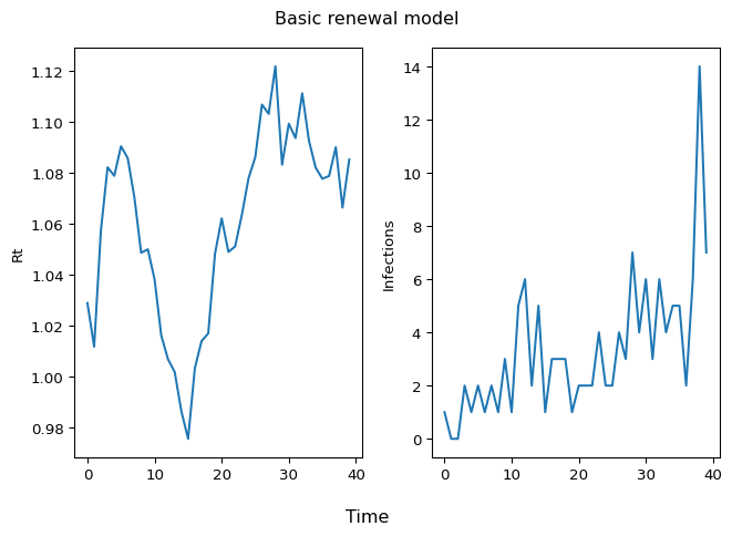
Figure 1: Rt and Infections

To fit the model, we can use the run() method of the RtInfectionsRenewalModel class (an inherited method from the metaclass Model). model1.run() will call the run method of the model1 object, which will generate an instance of model MCMC simulation, with 2000 warm-up iterations for the MCMC algorithm, used to tune the parameters of the MCMC algorithm to improve efficiency of the sampling process. From the posterior distribution of the model parameters, 1000 samples will be drawn and used to estimate the posterior distributions and compute summary statistics. Observed data is provided to the model using the sim_data object previously generated. mcmc_args provides additional arguments for the MCMC algorithm.

import jax

model1.run(
    num_warmup=2000,
    num_samples=1000,
    data_observed_infections=sim_data.observed_infections,
    rng_key=jax.random.key(54),
    mcmc_args=dict(progress_bar=False, num_chains=2),
)

Now, let’s investigate the output, particularly the posterior distribution of the \(\mathcal{R}(t)\) estimates:

import arviz as az

# Create arviz inference data object
idata = az.from_numpyro(
    posterior=model1.mcmc,
)

# Extract Rt signal samples across chains
rt = az.extract(idata.posterior["Rt"], num_samples=100)["Rt"].values


# Plot Rt signal
fig, ax = plt.subplots(1, 1, figsize=(8, 6))
ax.plot(
    np.arange(rt.shape[0]),
    rt,
    color="skyblue",
    alpha=0.10,
)
ax.plot([], [], color="skyblue", alpha=0.05, label="Rt Posterior Samples")
ax.plot(
    np.arange(rt.shape[0]),
    rt.mean(axis=1),
    color="black",
    linewidth=2.0,
    linestyle="--",
    label="Sample Mean",
)
ax.legend(loc="best")
ax.set_ylabel(r"$\mathscr{R}_t$ Signal", fontsize=20)
ax.set_xlabel("Days", fontsize=20)
plt.show()

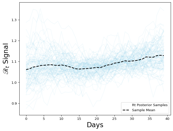
Figure 2: Rt posterior distribution

We can use the get_samples method to extract samples from the model

Rt_samp = model1.mcmc.get_samples()["Rt"]
latent_infection_samp = model1.mcmc.get_samples()["all_latent_infections"]

We can also convert the fitted model to ArviZ InferenceData object and use ArviZ package to extarct samples, calculate statistics, create model diagnostics and visualizations.

import arviz as az

idata = az.from_numpyro(model1.mcmc)

and use the InferenceData to compute the model-fit diagnostics. Here, we show diagnostic summary for the first 10 effective reproduction number \(\mathcal{R}(t)\).

diagnostic_stats_summary = az.summary(
    idata.posterior["Rt"][::, ::, 4:],  # ignore nan padding
    kind="diagnostics",
)

print(diagnostic_stats_summary)

        mcse_mean  mcse_sd  ess_bulk  ess_tail  r_hat
Rt[4]       0.002    0.003    1427.0     950.0   1.01
Rt[5]       0.002    0.003    1385.0     784.0   1.02
Rt[6]       0.002    0.003    1292.0     744.0   1.01
Rt[7]       0.002    0.003    1312.0     761.0   1.02
Rt[8]       0.002    0.003    1097.0     579.0   1.01
Rt[9]       0.002    0.003    1145.0     652.0   1.01
Rt[10]      0.001    0.002    1280.0     775.0   1.01
Rt[11]      0.001    0.002    1647.0     939.0   1.01
Rt[12]      0.001    0.002    1894.0     891.0   1.01
Rt[13]      0.001    0.002    1604.0     633.0   1.01
Rt[14]      0.001    0.003    1173.0     692.0   1.01
Rt[15]      0.002    0.002     625.0     469.0   1.01
Rt[16]      0.002    0.002     566.0     694.0   1.01
Rt[17]      0.002    0.002     398.0     592.0   1.01
Rt[18]      0.003    0.002     295.0     542.0   1.01
Rt[19]      0.002    0.002     328.0     472.0   1.01
Rt[20]      0.002    0.002     448.0     598.0   1.01
Rt[21]      0.002    0.003     607.0     511.0   1.01
Rt[22]      0.001    0.003     911.0     482.0   1.02
Rt[23]      0.001    0.002    1564.0     568.0   1.01
Rt[24]      0.001    0.002    2295.0     863.0   1.01
Rt[25]      0.001    0.002    2789.0     685.0   1.01
Rt[26]      0.001    0.002    3396.0     695.0   1.01
Rt[27]      0.001    0.002    3006.0     698.0   1.01
Rt[28]      0.001    0.002    2551.0     869.0   1.01
Rt[29]      0.001    0.002    1783.0     878.0   1.00
Rt[30]      0.001    0.002    2108.0     825.0   1.00
Rt[31]      0.001    0.002    1586.0    1230.0   1.00
Rt[32]      0.001    0.002    1275.0     657.0   1.01
Rt[33]      0.001    0.002    1036.0     504.0   1.00
Rt[34]      0.002    0.002     821.0     984.0   1.01
Rt[35]      0.002    0.002     668.0     636.0   1.00
Rt[36]      0.002    0.002     669.0     775.0   1.00
Rt[37]      0.003    0.003     471.0     709.0   1.01
Rt[38]      0.004    0.003     357.0     410.0   1.00
Rt[39]      0.004    0.004     468.0     663.0   1.01

Below we use plot_trace to inspect the trace of the first 10 inferred \(\mathcal{R}(t)\) values.

plt.rcParams["figure.constrained_layout.use"] = True

az.plot_trace(
    idata.posterior,
    var_names=["Rt"],
    coords={"Rt_dim_0": np.arange(4, 14)},
    compact=False,
)
plt.show()

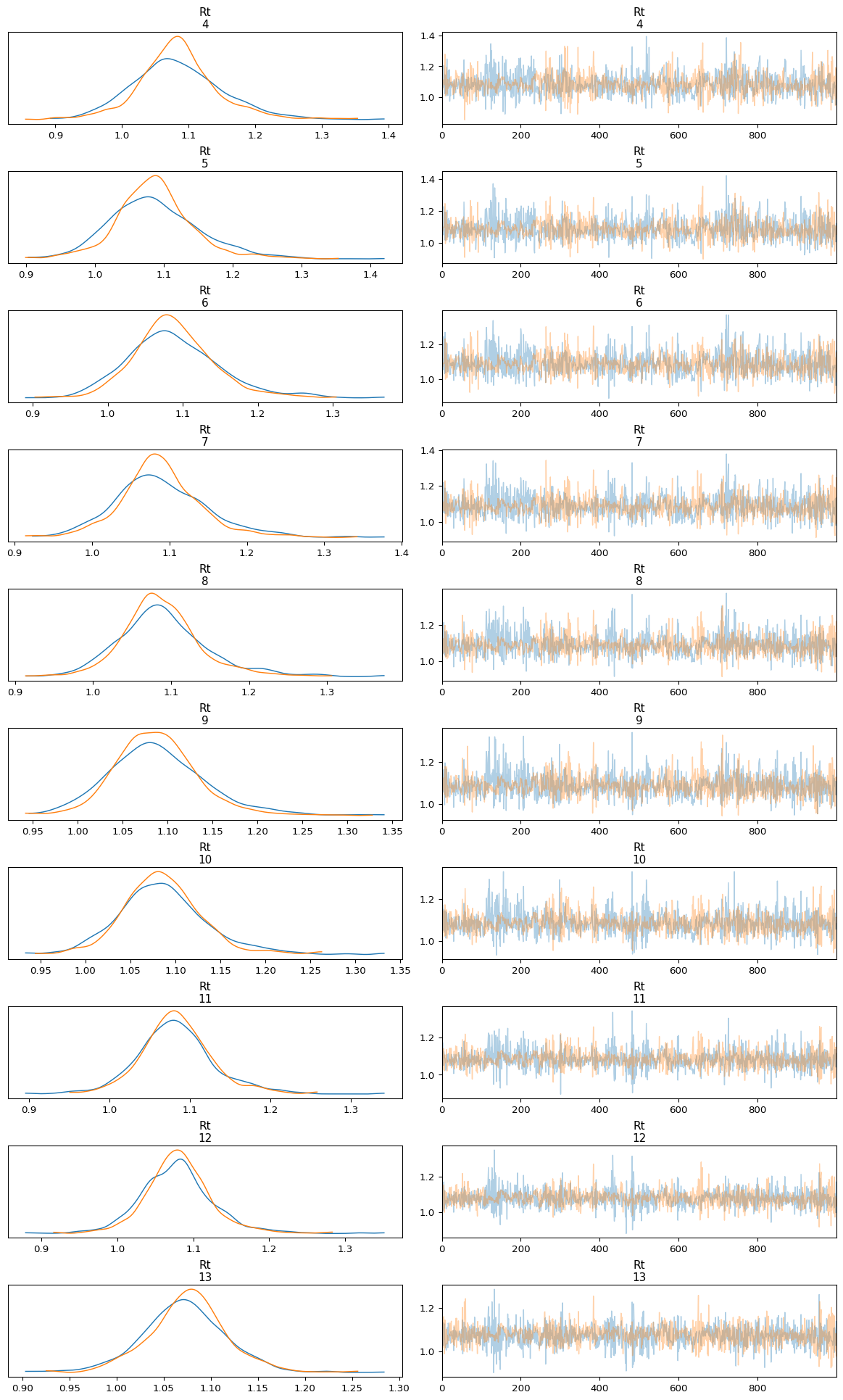
Figure 3: Trace plot of Rt posterior distribution

We inspect the posterior distribution of \(\mathcal{R}(t)\) by plotting the 90% and 50% highest density intervals:

x_data = idata.posterior["Rt_dim_0"][4:]
y_data = idata.posterior["Rt"][::, ::, 4:]

fig, axes = plt.subplots(figsize=(6, 5))
az.plot_hdi(
    x_data,
    y_data,
    hdi_prob=0.9,
    color="C0",
    fill_kwargs={"alpha": 0.3},
    ax=axes,
)

az.plot_hdi(
    x_data,
    y_data,
    hdi_prob=0.5,
    color="C0",
    fill_kwargs={"alpha": 0.6},
    ax=axes,
)

# Add mean of the posterior to the figure
median_ts = y_data.median(dim=["chain", "draw"])
axes.plot(x_data, median_ts, color="C0", label="Median")
axes.legend()
axes.set_title("Posterior Effective Reproduction Number", fontsize=10)
axes.set_xlabel("Time", fontsize=10)
axes.set_ylabel("$\\mathcal{R}(t)$", fontsize=10)
plt.show()

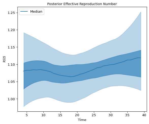
Figure 4: High density interval for Effective Reproduction Number

and latent infections:

x_data = idata.posterior["all_latent_infections_dim_0"]
y_data = idata.posterior["all_latent_infections"]

fig, axes = plt.subplots(figsize=(6, 5))
az.plot_hdi(
    x_data,
    y_data,
    hdi_prob=0.9,
    color="C0",
    smooth=False,
    fill_kwargs={"alpha": 0.3},
    ax=axes,
)

az.plot_hdi(
    x_data,
    y_data,
    hdi_prob=0.5,
    color="C0",
    smooth=False,
    fill_kwargs={"alpha": 0.6},
    ax=axes,
)

# plot the posterior median
median_ts = y_data.median(dim=["chain", "draw"])
axes.plot(x_data, median_ts, color="C0", label="Median")

axes.legend()
axes.set_title("Posterior Latent Infections", fontsize=10)
axes.set_xlabel("Time", fontsize=10)
axes.set_ylabel("Latent Infections", fontsize=10)
plt.show()

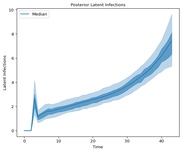
Figure 5: High density interval for Latent Infections

Fitting a basic renewal model

pyrenew core metaclasses

Architecture of RtInfectionsRenewalModel

Implementing a RtInfectionsRenewalModel

`pyrenew` core metaclasses

Architecture of `RtInfectionsRenewalModel`

Implementing a `RtInfectionsRenewalModel`