Implementing a Day of the Week Effect

This document illustrates how to leverage the time-aware arrays to create a a day of the week effect. We use the same model designed in the hospital admissions-only tutorial.

Recap: Hospital Admissions Model

In the “Fitting a hospital admissions-only model” tutorial, we built a fairly complicated model that included pre-defined random variables as well as a custom random variable representing the reproductive number.

flowchart LR

  %% Elements
  rt_proc["Random walk RT process <br/> (latent)"];
  latent_inf["Latent infections"]
  latent_ihr["Infection to hospitalization rate <br/> (latent)"]
  neg_binom["Observation process <br/> (hospitalizations)"]
  latent_hosp["Latent hospitalizations"];
  i0["Initial infections <br/> (latent)"];
  gen_int["Generation interval <br/> (fixed)"];
  hosp_int["Hospitalization interval <br/> (fixed)"];

  %% Models
  basic_model(("Infections model"));
  admin_model(("Hospital admissions model"));

  %% Latent infections
  rt_proc --> latent_inf;
  i0 --> latent_inf;
  gen_int --> latent_inf;
  latent_inf --> basic_model

  %% Hospitalizations
  hosp_int --> latent_hosp

  neg_binom --> admin_model;
  latent_ihr --> latent_hosp;
  basic_model --> admin_model;
  latent_hosp --> admin_model;

In this tutorial, we will focus on adding a new component: the day-of-the-week effect.

Setup: import all packages and load the simulated data

import numpyro
import polars as pl
import jax.numpy as jnp
import numpyro.distributions as dist
from pyrenew import (
    datasets,
    deterministic,
    latent,
    metaclass,
    model,
    observation,
    process,
    randomvariable,
    transformation,
)
from pyrenew.latent import (
    InfectionInitializationProcess,
    InitializeInfectionsExponentialGrowth,
)

numpyro.set_host_device_count(2)

# Loading and processing the data
dat = (
    datasets.load_wastewater()
    .group_by("date")
    .first()
    .select(["date", "daily_hosp_admits"])
    .sort("date")
    .head(90)
)
daily_hosp_admits = dat["daily_hosp_admits"].to_numpy()
dates = dat["date"].to_numpy()

# Loading additional datasets
gen_int = datasets.load_generation_interval()
inf_hosp_int = datasets.load_infection_admission_interval()

# We only need the probability_mass column of each dataset
gen_int_array = gen_int["probability_mass"].to_numpy()
inf_hosp_int_array = inf_hosp_int["probability_mass"].to_numpy()

/home/runner/work/PyRenew/PyRenew/.venv/lib/python3.13/site-packages/tqdm/auto.py:21: TqdmWarning: IProgress not found. Please update jupyter and ipywidgets. See https://ipywidgets.readthedocs.io/en/stable/user_install.html
  from .autonotebook import tqdm as notebook_tqdm

Define all model components

We start by (re)defining the hospital admissions model without a day-of-the-week effect.

# Hospital admissions
inf_hosp_int = deterministic.DeterministicPMF(
    name="inf_hosp_int", value=inf_hosp_int_array
)

hosp_rate = randomvariable.DistributionalVariable(
    name="IHR", distribution=dist.LogNormal(jnp.log(0.05), jnp.log(1.1))
)

latent_hosp = latent.HospitalAdmissions(
    infection_to_admission_interval_rv=inf_hosp_int,
    infection_hospitalization_ratio_rv=hosp_rate,
)


# Infection process
latent_inf = latent.Infections()
n_initialization_points = max(gen_int_array.size, inf_hosp_int_array.size) - 1

I0 = InfectionInitializationProcess(
    "I0_initialization",
    randomvariable.DistributionalVariable(
        name="I0",
        distribution=dist.LogNormal(loc=jnp.log(100), scale=jnp.log(1.75)),
    ),
    InitializeInfectionsExponentialGrowth(
        n_initialization_points,
        deterministic.DeterministicVariable(name="rate", value=0.05),
    ),
)

# Generation interval
gen_int_pmf = deterministic.DeterministicPMF(
    name="gen_int", value=gen_int_array
)


class RtRandomWalk(metaclass.RandomVariable):
    def validate(self):
        pass

    def sample(self, n: int, **kwargs) -> tuple:
        sd_rt = numpyro.sample("Rt_random_walk_sd", dist.HalfNormal(0.025))

        # Random walk step
        step_rv = randomvariable.DistributionalVariable(
            name="rw_step_rv", distribution=dist.Normal(0, sd_rt)
        )

        rt_init_rv = randomvariable.DistributionalVariable(
            name="init_log_rt", distribution=dist.Normal(0, 0.2)
        )

        # Random walk process
        base_rv = process.RandomWalk(
            name="log_rt",
            step_rv=step_rv,
        )

        # Transforming the random walk to the Rt scale
        rt_rv = randomvariable.TransformedVariable(
            name="Rt_rv",
            base_rv=base_rv,
            transforms=transformation.ExpTransform(),
        )
        init_rt = rt_init_rv.sample()

        return rt_rv.sample(n=n, init_vals=init_rt, **kwargs)


rtproc = RtRandomWalk()

# we place a log-Normal prior on the concentration
# parameter of the negative binomial.
nb_conc_rv = randomvariable.TransformedVariable(
    "concentration",
    randomvariable.DistributionalVariable(
        name="concentration_raw",
        distribution=dist.TruncatedNormal(loc=0, scale=1, low=0.01),
    ),
    transformation.PowerTransform(-2),
)

# now we define the observation process
obs = observation.NegativeBinomialObservation(
    "negbinom_rv",
    concentration_rv=nb_conc_rv,
)

# now we build the model
hosp_model = model.HospitalAdmissionsModel(
    latent_infections_rv=latent_inf,
    latent_hosp_admissions_rv=latent_hosp,
    I0_rv=I0,
    gen_int_rv=gen_int_pmf,
    Rt_process_rv=rtproc,
    hosp_admission_obs_process_rv=obs,
)

We run the model and then plot the posterior samples.

import jax
import numpy as np

# Model without weekday effect
hosp_model.run(
    num_samples=2000,
    num_warmup=2000,
    data_observed_hosp_admissions=daily_hosp_admits,
    rng_key=jax.random.key(54),
    mcmc_args=dict(progress_bar=False),
)

Code

import arviz as az
import matplotlib.pyplot as plt

ppc_samples = hosp_model.posterior_predictive(
    n_datapoints=daily_hosp_admits.size
)
idata = az.from_numpyro(
    posterior=hosp_model.mcmc,
    posterior_predictive=ppc_samples,
)

# Use a time series plot (plot_ts) from arviz for plotting
axes = az.plot_ts(
    idata,
    y="negbinom_rv",
    y_hat="negbinom_rv",
    num_samples=200,
    y_kwargs={
        "color": "blue",
        "linewidth": 1.0,
        "marker": "o",
        "linestyle": "solid",
    },
    y_hat_plot_kwargs={"color": "skyblue", "alpha": 0.05},
    y_mean_plot_kwargs={"color": "black", "linestyle": "--", "linewidth": 2.5},
    backend_kwargs={"figsize": (8, 6)},
    textsize=15.0,
)
ax = axes[0][0]
ax.set_xlabel("Time", fontsize=20)
ax.set_ylabel("Hospital Admissions", fontsize=20)
handles, labels = ax.get_legend_handles_labels()
ax.legend(
    handles, ["Observed", "Sample Mean", "Posterior Samples"], loc="best"
)
plt.show()

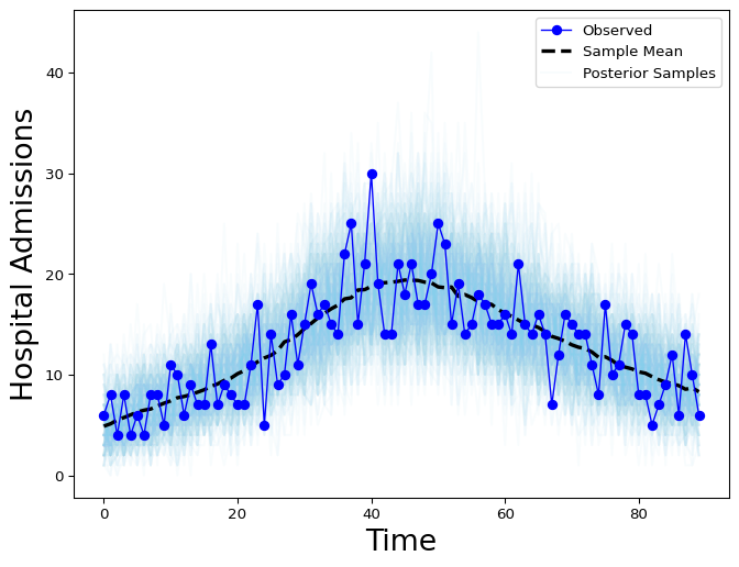
Figure 1: Hospital Admissions posterior distribution without weekday effect

Round 2: Incorporating day-of-the-week effects

To add a day-of-the-week effect to the previous model we add two additional arguments to the latent hospital admissions random variable:

• day_of_the_week_rv (a RandomVariable)
• obs_data_first_day_of_the_week (an int mapping days of the week from 0:6, zero being Monday).

The day_of_the_week_rv’s sample method should return a vector of length seven; those values are then broadcasted to match the length of the dataset. Since the observed data may start in a weekday other than Monday, the obs_data_first_day_of_the_week argument is used to offset the day-of-the-week effect.

For this effect we use a scaled Dirichlet distribution, and define a TransformedVariable that samples an array of length seven from numpyro’s distributions.Dirichlet and applies a transformation.AffineTransform to scale it by seven. ¹:

# Instantiating the day-of-the-week effect
dayofweek_effect = randomvariable.TransformedVariable(
    name="dayofweek_effect",
    base_rv=randomvariable.DistributionalVariable(
        name="dayofweek_effect_raw",
        distribution=dist.Dirichlet(jnp.ones(7)),
    ),
    transforms=transformation.AffineTransform(
        loc=0, scale=7, domain=jnp.array([0, 1])
    ),
)

We use this day-of-the-week effect as the latent hospital admissions random variable.

Since the day-of-the-week effect takes into account the first day of the dataset, we need to determine the day of the week of the first observation. To do this, we convert the first date in the dataset to a datetime object and extract the day of the week:

# Figuring out the day of the week of the first observation
import datetime as dt

first_dow_in_data = dates[0].astype(dt.datetime).weekday()
first_dow_in_data  # zero

# Define the latent hospital admissions RV with the day-of-the-week effect
latent_hosp_wday_effect = latent.HospitalAdmissions(
    infection_to_admission_interval_rv=inf_hosp_int,
    infection_hospitalization_ratio_rv=hosp_rate,
    day_of_week_effect_rv=dayofweek_effect,
    # Concidirently, this is zero
    obs_data_first_day_of_the_week=first_dow_in_data,
)

# New model with day-of-the-week effect
hosp_model_dow = model.HospitalAdmissionsModel(
    latent_infections_rv=latent_inf,
    latent_hosp_admissions_rv=latent_hosp_wday_effect,
    I0_rv=I0,
    gen_int_rv=gen_int_pmf,
    Rt_process_rv=rtproc,
    hosp_admission_obs_process_rv=obs,
)

Running the model:

# Model with weekday effect
hosp_model_dow.run(
    num_samples=2000,
    num_warmup=2000,
    data_observed_hosp_admissions=daily_hosp_admits,
    rng_key=jax.random.key(54),
    mcmc_args=dict(progress_bar=False),
)

As a result, we can see the posterior distribution of our novel day-of-the-week effect:

Code

# Create an InferenceData object from hosp_model_dow
dow_idata = az.from_numpyro(
    posterior=hosp_model_dow.mcmc,
)

# Extract day of week effect (DOW)
dow_effect_raw = dow_idata.posterior["dayofweek_effect_raw"].squeeze().T
indices = np.random.choice(dow_effect_raw.shape[1], size=200, replace=False)
dow_plot_samples = dow_effect_raw[:, indices]
fig, ax = plt.subplots(1, 1, figsize=(8, 6))
ax.plot(
    np.arange(dow_effect_raw.shape[0]),
    dow_plot_samples,
    color="skyblue",
    alpha=0.10,
)
ax.plot([], [], color="skyblue", alpha=0.10, label="DOW Posterior Samples")
ax.plot(
    np.arange(dow_effect_raw.shape[0]),
    dow_plot_samples.mean(dim="draw"),
    color="black",
    linewidth=2.0,
    linestyle="--",
    label="Sample Mean",
)
ax.legend(loc="best")
ax.set_ylabel("Effect", fontsize=20)
ax.set_xlabel("Day Of Week", fontsize=20)
plt.show()

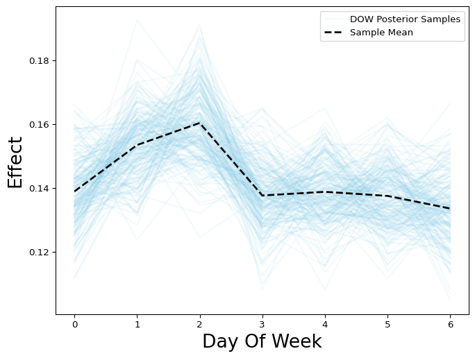
Figure 2: Day of the week effect

The new model with the day-of-the-week effect can be compared to the previous model, which doesn’t distinguish the day of the week, by plotting the posterior distributions from each.

Code

# Without weekday effect (from earlier)
axes = az.plot_ts(
    idata,
    y="negbinom_rv",
    y_hat="negbinom_rv",
    num_samples=200,
    y_kwargs={
        "color": "blue",
        "linewidth": 1.0,
        "marker": "o",
        "linestyle": "solid",
    },
    y_hat_plot_kwargs={"color": "skyblue", "alpha": 0.05},
    y_mean_plot_kwargs={"color": "black", "linestyle": "--", "linewidth": 2.5},
    backend_kwargs={"figsize": (8, 6)},
    textsize=15.0,
)
ax = axes[0][0]
ax.set_xlabel("Time", fontsize=20)
ax.set_ylabel("Hospital Admissions", fontsize=20)
handles, labels = ax.get_legend_handles_labels()
ax.legend(
    handles,
    ["Observed", "Posterior Predictive", "Samples wo/ WDE"],
    loc="best",
)
plt.show()

Figure 3: Hospital Admissions posterior distribution without weekday effect

Code

# Figure with weekday effect
ppc_samples = hosp_model_dow.posterior_predictive(
    n_datapoints=daily_hosp_admits.size
)
idata = az.from_numpyro(
    posterior=hosp_model_dow.mcmc,
    posterior_predictive=ppc_samples,
)

axes = az.plot_ts(
    idata,
    y="negbinom_rv",
    y_hat="negbinom_rv",
    num_samples=200,
    y_kwargs={
        "color": "blue",
        "linewidth": 1.0,
        "marker": "o",
        "linestyle": "solid",
    },
    y_hat_plot_kwargs={"color": "skyblue", "alpha": 0.05},
    y_mean_plot_kwargs={"color": "black", "linestyle": "--", "linewidth": 2.5},
    backend_kwargs={"figsize": (8, 6)},
    textsize=15.0,
)
ax = axes[0][0]
ax.set_xlabel("Time", fontsize=20)
ax.set_ylabel("Hospital Admissions", fontsize=20)
handles, labels = ax.get_legend_handles_labels()
ax.legend(
    handles, ["Observed", "Posterior Predictive", "Samples w/ WDE"], loc="best"
)
plt.show()

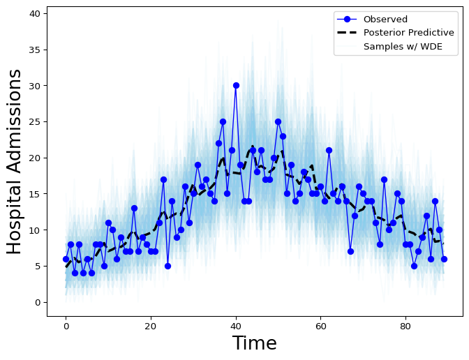
Figure 4: Hospital Admissions posterior distribution with weekday effect

---

1. A similar weekday effect is implemented in its own module, with example code in the Periodic Effects tutorial. ↩