State-Level NHSN Nowcasts

Quick Example

Here’s a complete working example using test mode (fast configuration for demonstration):

library(nowcastNHSN)
library(dplyr)

# Create test configuration (single state, few draws for speed)
config <- nowcast_config_test(location = "ca", draws = 10)
print(config)

# Fetch data for California
source <- delphi_epidata_source(target = "covid", geo_types = "state")
reporting_data <- fetch_reporting_data(
  source = source,
  reference_dates = epidatr::epirange(202450, 202510),
  report_dates = epidatr::epirange(202450, 202512),
  locations = "ca"
)

# Run nowcast - conversion to incremental counts happens internally
results <- run_single_nowcast(
  data = reporting_data,
  location = "ca",
  config = config,
  nowcast_date = max(reporting_data$reference_date)
)
head(results, 10)
#>     pred_count reference_date draw output_type location
#> 1          723     2024-12-14    1     samples       ca
#> 13         723     2024-12-14    2     samples       ca
#> 25         723     2024-12-14    3     samples       ca
#> 37         723     2024-12-14    4     samples       ca
#> 49         723     2024-12-14    5     samples       ca
#> 61         723     2024-12-14    6     samples       ca
#> 73         723     2024-12-14    7     samples       ca
#> 85         723     2024-12-14    8     samples       ca
#> 97         723     2024-12-14    9     samples       ca
#> 109        723     2024-12-14   10     samples       ca

# Summarize to forecast hub format
summary <- summarize_nowcast(results)
head(summary)
#> # A tibble: 6 × 5
#>   reference_date location output_type output_type_id value
#>   <date>         <chr>    <chr>       <chr>          <dbl>
#> 1 2024-12-14     ca       quantile    0.01             723
#> 2 2024-12-14     ca       quantile    0.025            723
#> 3 2024-12-14     ca       quantile    0.05             723
#> 4 2024-12-14     ca       quantile    0.1              723
#> 5 2024-12-14     ca       quantile    0.15             723
#> 6 2024-12-14     ca       quantile    0.2              723

library(ggplot2)

# Pivot quantiles to wide format for ribbon plot
quantile_wide <- summary |>
  tidyr::pivot_wider(
    names_from = output_type_id,
    values_from = value,
    names_prefix = "q"
  )

nowcast_date <- max(reporting_data$reference_date)

# Get counts at nowcast time (incomplete)
at_nowcast_time <- reporting_data |>
  filter(location == "ca", report_date <= nowcast_date) |>
  group_by(reference_date) |>
  filter(report_date == max(report_date)) |>
  ungroup() |>
  select(reference_date, at_nowcast = count)

# Get final reported counts (from latest available data)
final_reported <- reporting_data |>
  filter(location == "ca") |>
  group_by(reference_date) |>
  filter(report_date == max(report_date)) |>
  ungroup() |>
  select(reference_date, final = count)

# Join all data
plot_data <- quantile_wide |>
  left_join(at_nowcast_time, by = "reference_date") |>
  left_join(final_reported, by = "reference_date")

# Create nowcast visualization
ggplot(plot_data, aes(x = reference_date)) +
  # Prediction intervals (draw first so behind)
  geom_ribbon(aes(ymin = q0.05, ymax = q0.95, fill = "90% Prediction Interval"), alpha = 0.3) +
  # At nowcast time

  geom_point(aes(y = at_nowcast, color = "At Nowcast Time"), size = 2) +
  geom_line(aes(y = at_nowcast, color = "At Nowcast Time"), linewidth = 1) +
  # Nowcast median
  geom_point(aes(y = q0.5, color = "Nowcast (Median)"), size = 2, shape = 17) +
  geom_line(aes(y = q0.5, color = "Nowcast (Median)"), linewidth = 1, linetype = "dashed") +
  # Final reported
  geom_point(aes(y = final, color = "Final Reported"), size = 2, shape = 15) +
  geom_line(aes(y = final, color = "Final Reported"), linewidth = 1, linetype = "dotted") +
  labs(
    title = "COVID-19 Nowcast for California",
    subtitle = "Comparing nowcast predictions with counts at nowcast time and final values",
    x = "Reference Date",
    y = "Count",
    color = "Count Type",
    fill = NULL
  ) +
  theme_minimal() +
  theme(
    axis.text.x = element_text(angle = 45, hjust = 1),
    legend.position = "bottom"
  ) +
  scale_color_manual(values = c(
    "At Nowcast Time" = "#E41A1C",
    "Nowcast (Median)" = "#377EB8",
    "Final Reported" = "#4DAF4A"
  )) +
  scale_fill_manual(values = c("90% Prediction Interval" = "#377EB8"))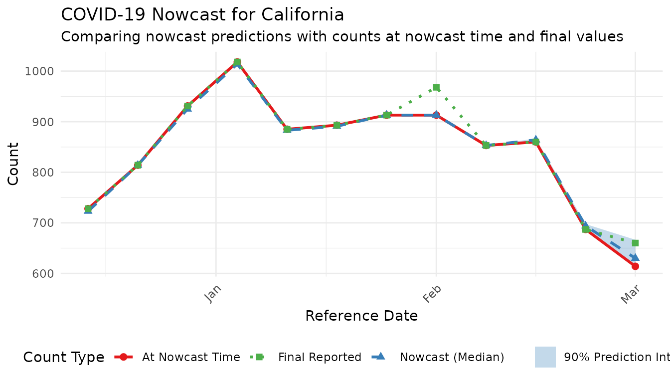

The rest of this vignette provides detailed documentation for production use.

Introduction

This vignette demonstrates how to run NHSN nowcasts for multiple US states/territories using the nowcastNHSN package. The workflow supports:

• Batch processing: Run nowcasts for all states in one call
• Single-state execution: Process individual states (useful for Azure task parallelization)
• Configurable parameters: Customize max_delay, scale_factor, prop_delay, and uncertainty models
• Partitioned parquet output: Efficient storage and querying with arrow

Setup

library(nowcastNHSN)
library(baselinenowcast)
library(dplyr)
library(ggplot2)

Configuration

The nowcast_config() function creates a validated configuration object with nowcast parameters:

# Default configuration
config <- nowcast_config()
print(config)

# Custom configuration
config <- nowcast_config(
  max_delay = 5,
  scale_factor = 3,
  prop_delay = 0.5,
  uncertainty_model = "skellam",  # Options: "negative_binomial", "normal", "skellam"
  draws = 500,
  output_dir = "output/nowcasts"
)

# Location-specific overrides (optional)
# These override the default config for specific locations
location_configs <- list(
  ca = nowcast_config(max_delay = 5, draws = 500),
  ny = nowcast_config(max_delay = 7, uncertainty_model = "normal", draws = 500)
)
# Other locations will use the default config

Configuration Parameters

Parameter	Description	Default
max_delay	Maximum reporting delay in weeks	7
scale_factor	Multiplier on max_delay for training volume	3
prop_delay	Proportion of training data for delay estimation	0.5
uncertainty_model	Error distribution: "negative_binomial", "normal", "skellam"	"negative_binomial"
draws	Number of posterior samples	1000
location	Single location code (optional)	NULL
output_dir	Directory for parquet output	NULL

Fetching Data

Fetch reporting data for all states in a single API call:

# Create data source
source <- delphi_epidata_source(
  target = "covid",
  geo_types = "state"
)

# Define date ranges
reference_dates <- epidatr::epirange(202450, 202510)
report_dates <- epidatr::epirange(202450, 202512)

# Fetch all states at once (efficient - single API call)
reporting_data <- fetch_reporting_data(
  source = source,
  reference_dates = reference_dates,
  report_dates = report_dates,
  locations = "*"  # All locations
)

# Convert cumulative to incremental counts
incremental_data <- cumulative_to_incremental(
  reporting_data,
  group_cols = c("reference_date", "location", "signal")
)

head(incremental_data)

Running Nowcasts

Batch Processing (All States)

# Configure nowcast parameters
config <- nowcast_config(
  draws = 100,
  output_dir = "output/nowcasts"
)

# Run nowcasts for all states
# This filters the pre-fetched data per state, runs baselinenowcast, and combines results
results <- run_state_nowcasts(
  data = incremental_data,
  config = config,
  locations = "all"
)

# Check for any failures
failed_locations <- attr(results, "failed_locations")
if (length(failed_locations) > 0) {
  message("Failed locations: ", paste(failed_locations, collapse = ", "))
}

# View results structure
head(results)

Single-State Execution

For Azure task parallelization, you can run individual states:

config <- nowcast_config(
  uncertainty_model = "normal",
  draws = 100
)

# Run for a single state
ca_results <- run_single_nowcast(
  data = incremental_data,
  location = "ca",
  config = config,
  nowcast_date = max(incremental_data$reference_date)
)

head(ca_results)

Location-Specific Configurations

Use location_configs to override settings for specific locations while using a default for the rest:

# Default config for most states
default_config <- nowcast_config(max_delay = 7, draws = 100)

# Overrides for states that need different settings
location_configs <- list(
  ca = nowcast_config(max_delay = 5, draws = 100),
  ny = nowcast_config(max_delay = 7, uncertainty_model = "normal", draws = 100)
)

results <- run_state_nowcasts(
  data = incremental_data,
  config = default_config,
  location_configs = location_configs,
  locations = c("ca", "ny", "tx")  # tx uses default_config
)

Parallel Processing

Enable parallel processing for faster batch runs:

library(future)
plan(multisession, workers = 4)

config <- nowcast_config(
  draws = 100
)

results <- run_state_nowcasts(
  data = incremental_data,
  config = config,
  locations = "all",
  parallel = TRUE
)

Output

Summarizing Results

Convert raw draws to quantile summaries:

summary <- summarize_nowcast(results)
head(summary)

Writing to Parquet

Results are written as partitioned parquet files for efficient querying:

# Write summarized results (default)
write_nowcast_parquet(results, "output/nowcasts")

# Write raw draws instead
write_nowcast_parquet(results, "output/nowcasts_draws", summarize = FALSE)

This creates a directory structure like:

output/nowcasts/
├── location=ca/
│   └── part-0.parquet
├── location=ny/
│   └── part-0.parquet
└── location=tx/
    └── part-0.parquet

Reading Parquet Results

library(arrow)

# Read all locations
all_results <- read_nowcast_parquet("output/nowcasts")

# Read specific locations (efficient - only reads needed partitions)
ca_ny <- read_nowcast_parquet("output/nowcasts", locations = c("ca", "ny"))

# Or use arrow directly for more control
ds <- open_dataset("output/nowcasts")
ds |>
  filter(location == "ca", reference_date >= "2025-01-01") |>
  collect()

Command Line Usage

The package includes an entrypoint script for Azure or batch execution:

# Run all states
Rscript inst/scripts/run_nowcast.R --location all --output-dir output/nowcasts

# Run single state (for Azure task)
Rscript inst/scripts/run_nowcast.R --location ca --output-dir output/nowcasts

# Custom parameters
Rscript inst/scripts/run_nowcast.R \
  --location ca,ny,tx \
  --uncertainty-model skellam \
  --max-delay 5 \
  --draws 500 \
  --output-dir output/nowcasts \
  --parallel

# Show help
Rscript inst/scripts/run_nowcast.R --help

Visualizing Results

# Get summary for selected states
summary <- summarize_nowcast(results) |>
  filter(location %in% c("ca", "ny", "tx"))

ggplot(summary, aes(x = reference_date)) +
  geom_ribbon(aes(ymin = q05, ymax = q95, fill = location), alpha = 0.2) +
  geom_ribbon(aes(ymin = q25, ymax = q75, fill = location), alpha = 0.4) +
  geom_line(aes(y = median, color = location), linewidth = 1) +
  facet_wrap(~location, scales = "free_y", ncol = 1) +
  labs(
    title = "NHSN COVID-19 Nowcasts by State",
    subtitle = "Median with 50% and 90% prediction intervals",
    x = "Reference Date",
    y = "Predicted Admissions",
    color = "State",
    fill = "State"
  ) +
  theme_minimal() +
  theme(legend.position = "none")

Error Handling

The pipeline wraps each state’s nowcast in error handling, allowing the batch to continue even if individual states fail:

results <- run_state_nowcasts(data, config)

# Check which states failed
failed <- attr(results, "failed_locations")

if (length(failed) > 0) {
  warning("The following states failed: ", paste(failed, collapse = ", "))
  # Results still contain successful states
}

Common failure causes: - Insufficient data for a state (not enough reference dates) - Data quality issues (all zeros, excessive missing values) - Numerical issues in uncertainty estimation

Uncertainty Models

The package supports three uncertainty models:

Negative Binomial (Default)

Best for count data with overdispersion. Cannot produce negative predictions.

config <- nowcast_config(uncertainty_model = "negative_binomial")

Normal (Rounded)

Symmetric uncertainty around point predictions. Rounds to integers. Can produce negative values for small counts.

config <- nowcast_config(uncertainty_model = "normal")

Skellam

Difference of two Poissons. Naturally handles negative revisions. Good for data with frequent downward corrections.

config <- nowcast_config(uncertainty_model = "skellam")