Pyrenew demo#
This demo simulates a basic renewal process data and then fits it using
pyrenew.
You’ll need to install pyrenew using either poetry or pip. To
install pyrenew using poetry, run the following command from within
the directory containing the pyrenew project:
poetry install
To install pyrenew using pip, run the following command:
pip install git+https://github.com/CDCgov/multisignal-epi-inference@main#subdirectory=model
To begin, run the following import section to call external modules and
functions necessary to run the pyrenew demo. The import
statement imports the module and the as statement renames the module
for use within this script. The from statement imports a specific
function from a module (named after the .) within a package (named
before the .).
import matplotlib as mpl
import matplotlib.pyplot as plt
import jax
import jax.numpy as jnp
import numpy as np
from numpyro.handlers import seed
import numpyro.distributions as dist
from pyrenew.process import SimpleRandomWalkProcess
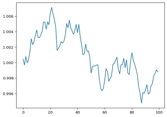
To understand the simple random walk process underlying the sampling
within the renewal process model, we first examine a single random walk
path. Using the sample method from an instance of the
SimpleRandomWalkProcess class, we first create an instance of the
SimpleRandomWalkProcess class with a normal distribution of mean = 0
and standard deviation = 0.0001 as its input. Next, the with
statement sets the seed for the random number generator for the
n_timepoints of the block that follows. Inside the with block, the
q_samp = q.sample(n_timepoints=100) generates the sample instance
over a n_timepoints of 100 time units. Finally, this single random walk
process is visualized using matplot.pyplot to plot the exponential
of the sample instance.
np.random.seed(3312)
q = SimpleRandomWalkProcess(dist.Normal(0, 0.001))
with seed(rng_seed=np.random.randint(0, 1000)):
    q_samp = q.sample(n_timepoints=100)

plt.plot(np.exp(q_samp[0]))
Next, import several additional functions from the latent module of
the pyrenew package to model infections and hospital admissions.
from pyrenew.latent import (
    Infections,
    HospitalAdmissions,
)
from pyrenew.metaclass import DistributionalRV
Additionally, import several classes from Pyrenew, including a Poisson observation process, determininstic PMF and variable classes, the Pyrenew hospitalization model, and a renewal model (Rt) random walk process:
from pyrenew.observation import PoissonObservation
from pyrenew.deterministic import DeterministicPMF, DeterministicVariable
from pyrenew.model import HospitalAdmissionsModel
from pyrenew.process import RtRandomWalkProcess
from pyrenew.latent import InfectionSeedingProcess, SeedInfectionsZeroPad
import pyrenew.transformation as t
To initialize the model, we first define initial conditions, including:
deterministic generation time, defined as an instance of the
DeterministicPMFclass, which gives the probability of each possible outcome for a discrete random variable given as a JAX NumPy array of four possible outcomesinitial infections at the start of the renewal process as a log-normal distribution with mean = 0 and standard deviation = 1. Infections before this time are assumed to be 0.
latent infections as an instance of the
Infectionsclass with default settingslatent hospitalization process, modeled by first defining the time interval from infections to hospitalizations as a
DeterministicPMFinput with 18 possible outcomes and corresponding probabilities given by the values in the array. TheHospitalAdmissionsfunction then takes in this defined time interval, as well as defining the rate at which infections are admitted to the hospital due to infection, modeled as a log-normal distribution with mean =jnp.log(0.05)and standard deviation = 0.05.hospitalization observation process, modeled with a Poisson distribution
an Rt random walk process with default settings
# Initializing model components:

# 1) A deterministic generation time
pmf_array = jnp.array([0.25, 0.25, 0.25, 0.25])
gen_int = DeterministicPMF(pmf_array, name="gen_int")

# 2) Initial infections
I0 = InfectionSeedingProcess(
    "I0_seeding",
    DistributionalRV(dist=dist.LogNormal(0, 1), name="I0"),
    SeedInfectionsZeroPad(pmf_array.size),
)

# 3) The latent infections process
latent_infections = Infections()

# 4) The latent hospitalization process:

# First, define a deterministic infection to hosp pmf
inf_hosp_int = DeterministicPMF(
    jnp.array(
        [0, 0, 0, 0, 0, 0, 0, 0, 0, 0, 0, 0, 0, 0.25, 0.5, 0.1, 0.1, 0.05]
    ),
    name="inf_hosp_int",
)

latent_admissions = HospitalAdmissions(
    infection_to_admission_interval_rv=inf_hosp_int,
    infect_hosp_rate_rv=DistributionalRV(
        dist=dist.LogNormal(jnp.log(0.05), 0.05), name="IHR"
    ),
)

# 5) An observation process for the hospital admissions
admissions_process = PoissonObservation()

# 6) A random walk process (it could be deterministic using
# pyrenew.process.DeterministicProcess())
Rt_process = RtRandomWalkProcess(
    Rt0_dist=dist.TruncatedNormal(loc=1.2, scale=0.2, low=0),
    Rt_transform=t.ExpTransform().inv,
    Rt_rw_dist=dist.Normal(0, 0.025),
)
The HospitalAdmissionsModel is then initialized using the initial
conditions just defined:
# Initializing the model
hospmodel = HospitalAdmissionsModel(
    gen_int_rv=gen_int,
    I0_rv=I0,
    latent_hosp_admissions_rv=latent_admissions,
    hosp_admission_obs_process_rv=admissions_process,
    latent_infections_rv=latent_infections,
    Rt_process_rv=Rt_process,
)
Next, we sample from the hospmodel for 30 time steps and view the
output of a single run:
with seed(rng_seed=np.random.randint(1, 60)):
    x = hospmodel.sample(n_timepoints_to_simulate=30)
x
/home/runner/.cache/pypoetry/virtualenvs/pyrenew-ay_vsbmF-py3.12/lib/python3.12/site-packages/jax/_src/numpy/lax_numpy.py:3044: FutureWarning: None encountered in jnp.array(); this is currently treated as NaN. In the future this will result in an error.
  return array(arys[0], copy=False, ndmin=1)
HospModelSample(Rt=[      nan       nan       nan       nan 1.1791104 1.1995267 1.1772177
 1.1913829 1.2075942 1.1444623 1.1514508 1.1976782 1.2292639 1.1719677
 1.204649  1.2323451 1.2466507 1.2800207 1.2749145 1.2520573 1.2094396
 1.2097179 1.2193931 1.2033775 1.1814811 1.2079672 1.1847589 1.1989986
 1.1871533 1.2152797 1.2211653 1.2328914 1.2036034 1.1977075], latent_infections=[0.         0.         0.         0.17688063 0.05214045 0.06867922
 0.08761451 0.11476436 0.09757317 0.10547114 0.1167062  0.13010225
 0.13824694 0.14372033 0.15924728 0.17601486 0.19236736 0.21483542
 0.23664482 0.2566287  0.27226794 0.29649484 0.32375994 0.34571573
 0.36573884 0.4021653  0.42573714 0.4614217  0.4912034  0.5409598
 0.58595234 0.6409609  0.679758   0.73288655], infection_hosp_rate=[0.04929917], latent_hosp_admissions=[0.         0.         0.         0.         0.         0.
 0.         0.         0.         0.         0.         0.
 0.         0.         0.         0.         0.00218002 0.00500265
 0.0030037  0.0039018  0.00460574 0.0049305  0.00487205 0.00530097
 0.00576412 0.00624666 0.00665578 0.00711595 0.0078055  0.00854396
 0.00939666 0.01042083 0.01143744 0.01238137], observed_hosp_admissions=[0 0 0 0 0 0 0 0 0 0 0 0 0 0 0 0 0 0 0 0 0 0 0 0 0 0 0 0 0 0 0 0 0 0]
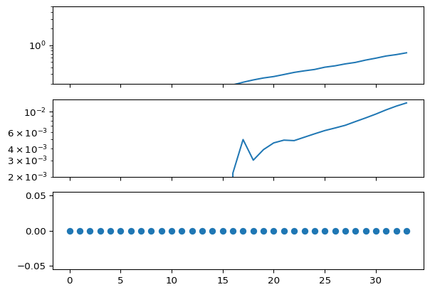
Visualizations of the single model output show (top) infections over the 30 time steps, (middle) hospital admissions over the 30 time steps, and observed hospital admissions (bottom)
fig, ax = plt.subplots(nrows=3, sharex=True)
ax[0].plot(x.latent_infections)
ax[0].set_ylim([1 / 5, 5])
ax[1].plot(x.latent_hosp_admissions)
ax[2].plot(x.observed_hosp_admissions, "o")
for axis in ax[:-1]:
    axis.set_yscale("log")
To fit the hospmodel to the simulated data, we call
hospmodel.run(), an MCMC algorithm, with the arguments generated in
hospmodel object, using 1000 warmup stepts and 1000 samples to draw
from the posterior distribution of the model parameters. The model is
run for len(x.sampled)-1 time steps with the seed set by
jax.random.PRNGKey()
# from numpyro.infer import MCMC, NUTS
hospmodel.run(
    num_warmup=1000,
    num_samples=1000,
    data_observed_hosp_admissions=x.observed_hosp_admissions,
    rng_key=jax.random.PRNGKey(54),
    mcmc_args=dict(progress_bar=False),
)
Print a summary of the model:
hospmodel.print_summary()
                                 mean       std    median      5.0%     95.0%     n_eff     r_hat
                         I0      0.82      0.79      0.60      0.02      1.70   1087.18      1.00
                        IHR      0.05      0.00      0.05      0.05      0.05   1724.84      1.00
                        Rt0      1.10      0.17      1.10      0.83      1.40   1611.03      1.00
 Rt_transformed_rw_diffs[0]     -0.00      0.03     -0.00     -0.05      0.04   1744.02      1.00
 Rt_transformed_rw_diffs[1]     -0.00      0.02     -0.00     -0.04      0.04   2643.43      1.00
 Rt_transformed_rw_diffs[2]     -0.00      0.02     -0.00     -0.04      0.04   1853.81      1.00
 Rt_transformed_rw_diffs[3]     -0.00      0.02     -0.00     -0.04      0.04   1673.03      1.00
 Rt_transformed_rw_diffs[4]     -0.00      0.02     -0.00     -0.04      0.03   2064.48      1.00
 Rt_transformed_rw_diffs[5]     -0.00      0.03     -0.00     -0.04      0.04   2023.50      1.00
 Rt_transformed_rw_diffs[6]      0.00      0.03      0.00     -0.04      0.04   2347.11      1.00
 Rt_transformed_rw_diffs[7]     -0.00      0.02     -0.00     -0.04      0.04   2079.08      1.00
 Rt_transformed_rw_diffs[8]     -0.00      0.03     -0.00     -0.05      0.04   1651.35      1.00
 Rt_transformed_rw_diffs[9]     -0.00      0.02     -0.00     -0.04      0.04   2218.48      1.00
Rt_transformed_rw_diffs[10]     -0.00      0.03     -0.00     -0.04      0.04   2533.24      1.00
Rt_transformed_rw_diffs[11]     -0.00      0.02     -0.00     -0.04      0.04   1447.84      1.00
Rt_transformed_rw_diffs[12]      0.00      0.02      0.00     -0.04      0.03   1816.49      1.00
Rt_transformed_rw_diffs[13]     -0.00      0.03     -0.00     -0.04      0.04   1863.06      1.00
Rt_transformed_rw_diffs[14]     -0.00      0.03     -0.00     -0.04      0.04   1667.84      1.00
Rt_transformed_rw_diffs[15]     -0.00      0.02     -0.00     -0.04      0.04   1778.66      1.00
Rt_transformed_rw_diffs[16]     -0.00      0.02     -0.00     -0.04      0.04   1531.03      1.00
Rt_transformed_rw_diffs[17]      0.00      0.03      0.00     -0.04      0.04   1649.99      1.00
Rt_transformed_rw_diffs[18]     -0.00      0.02     -0.00     -0.04      0.04   2350.43      1.00
Rt_transformed_rw_diffs[19]      0.00      0.02      0.00     -0.04      0.04   1262.52      1.00
Rt_transformed_rw_diffs[20]     -0.00      0.02     -0.00     -0.04      0.04   1480.42      1.00
Rt_transformed_rw_diffs[21]     -0.00      0.03      0.00     -0.04      0.04   1695.73      1.00
Rt_transformed_rw_diffs[22]      0.00      0.03      0.00     -0.04      0.04   1981.87      1.00
Rt_transformed_rw_diffs[23]     -0.00      0.03     -0.00     -0.05      0.04   1953.70      1.00
Rt_transformed_rw_diffs[24]      0.00      0.03      0.00     -0.04      0.04   1661.00      1.00
Rt_transformed_rw_diffs[25]     -0.00      0.02     -0.00     -0.04      0.04   2466.03      1.00
Rt_transformed_rw_diffs[26]      0.00      0.03      0.00     -0.04      0.04   1715.96      1.00
Rt_transformed_rw_diffs[27]     -0.00      0.02     -0.00     -0.04      0.04   1338.85      1.00
Rt_transformed_rw_diffs[28]     -0.00      0.02     -0.00     -0.04      0.04   1712.51      1.00
Rt_transformed_rw_diffs[29]      0.00      0.02      0.00     -0.04      0.04   1509.81      1.00
Rt_transformed_rw_diffs[30]      0.00      0.03      0.00     -0.04      0.04   1627.71      1.00
Rt_transformed_rw_diffs[31]      0.00      0.03      0.00     -0.04      0.04   1354.97      1.00
Rt_transformed_rw_diffs[32]      0.00      0.03      0.00     -0.04      0.05   1637.27      1.00

Number of divergences: 0
Next, we will use the spread_draws function from the
pyrenew.mcmcutils module to process the MCMC samples. The
spread_draws function reformats the samples drawn from the
mcmc.get_samples() from the hospmodel. The samples are simulated
Rt values over time.
from pyrenew.mcmcutils import spread_draws

samps = spread_draws(hospmodel.mcmc.get_samples(), [("Rt", "time")])
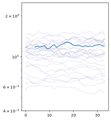
We visualize these samples below, with individual possible Rt estimates over time shown in light blue, and the overall mean estimate Rt shown in dark blue.
import numpy as np
import polars as pl

fig, ax = plt.subplots(figsize=[4, 5])

ax.plot(x[0])
samp_ids = np.random.randint(size=25, low=0, high=999)
for samp_id in samp_ids:
    sub_samps = samps.filter(pl.col("draw") == samp_id).sort(pl.col("time"))
    ax.plot(
        sub_samps.select("time").to_numpy(),
        sub_samps.select("Rt").to_numpy(),
        color="darkblue",
        alpha=0.1,
    )
ax.set_ylim([0.4, 1 / 0.4])
ax.set_yticks([0.5, 1, 2])
ax.set_yscale("log")