Getting started with pyrenew#

pyrenew is a flexible tool for simulating and making statistical inferences from epidemiologic models, with an emphasis on renewal models. Built on numpyro, pyrenew provides core components for model building and pre-defined models for processing various observational processes. This document illustrates how pyrenew can be used to build a basic renewal model.

The fundamentals#

pyrenew’s core components are the metaclasses RandomVariable and Model (in Python, a metaclass is a class whose instances are also classes, where a class is a template for making objects). Within the pyrenew package, a RandomVariable is a quantity that models can estimate and sample from, including deterministic quantities. The benefit of this design is that the definition of the sample() function can be arbitrary, allowing the user to either sample from a distribution using numpyro.sample(), compute fixed quantities (like a mechanistic equation), or return a fixed value (like a pre-computed PMF.) For instance, when estimating a PMF, the RandomVariable sampling function may roughly be defined as:

# define a new class called MyRandVar that inherits from the RandomVariable class
class MyRandVar(RandomVariable):
    #define a method called sample that returns an object of type ArrayLike
    def sample(...) -> ArrayLike:
        # calls sample function from NumPyro package
        return numpyro.sample(...)

Whereas, in some other cases, we may instead use a fixed quantity for that variable (like a pre-computed PMF), where the RandomVariable’s sample function could instead be defined as:

# instead define MyRandVar to still inherit from the RandVariable class
class MyRandVar(RandomVariable):
    #define sample method that still returns an ArrayLike object
    def sample(...) -> ArrayLike:
        #sampling method is a pre-computed PMF, a JAX NumPy array with explicit elements
        return jax.numpy.array([0.2, 0.7, 0.1])

Thus, when a Model samples from MyRandVar, it could be either adding random variables to be estimated (first case) or just retrieving some quantity needed for other calculations (second case.)

The Model metaclass provides basic functionality for estimating and simulation. Like RandomVariable, the Model metaclass has a sample() method that defines the model structure. Ultimately, models can be nested (or inherited), providing a straightforward way to add layers of complexity.

‘Hello world’ model#

This section will show the steps to build a simple renewal model featuring a latent infection process, a random walk Rt process, and an observation process for the reported infections.

We start by loading the needed components to build a basic renewal model:

import jax.numpy as jnp
import numpy as np
import numpyro as npro
import numpyro.distributions as dist
from pyrenew.process import RtRandomWalkProcess
from pyrenew.latent import (
    Infections,
    InfectionSeedingProcess,
    SeedInfectionsZeroPad,
)
from pyrenew.observation import PoissonObservation
from pyrenew.deterministic import DeterministicPMF
from pyrenew.model import RtInfectionsRenewalModel
from pyrenew.metaclass import DistributionalRV
import pyrenew.transformation as t

The pyrenew package models the real-time reproductive number \(R_t\), the ratio of new infections at time \(t\) to previous infections at some time \(t-s\), as a renewal process model. Our basic renewal process model defines five components:

generation interval, the times between infections
initial infections, occurring prior to time \(t = 0\)
\(R_t\), the real-time reproductive number,
latent infections, i.e., those infections which are known to exist but are not observed (or not observable), and
observed infections, a subset of underlying true infections that are reported, perhaps via hospital admissions, physician’s office visits, or routine biosurveillance.

To initialize these five components within the renewal modeling framework, we estimate each component with:

In this example, the generation interval is not estimated but passed as a deterministic instance of RandomVariable
an instance of the InfectionSeedingProcess class, where the number of latent infections immediately before the renewal process begins follows a log-normal distribution with mean = 0 and standard deviation = 1. By specifying SeedInfectionsZeroPad, the latent infections before this time are assumed to be 0.
an instance of the RtRandomWalkProcess class with default values
an instance of the Infections class with default values, and
an instance of the PoissonObservation class with default values

# (1) The generation interval (deterministic)
pmf_array = jnp.array([0.25, 0.25, 0.25, 0.25])
gen_int = DeterministicPMF(pmf_array, name="gen_int")

# (2) Initial infections (inferred with a prior)
I0 = InfectionSeedingProcess(
    "I0_seeding",
    DistributionalRV(dist=dist.LogNormal(0, 1), name="I0"),
    SeedInfectionsZeroPad(pmf_array.size),
)

# (3) The random process for Rt
rt_proc = RtRandomWalkProcess(
    Rt0_dist=dist.TruncatedNormal(loc=1.2, scale=0.2, low=0),
    Rt_transform=t.ExpTransform().inv,
    Rt_rw_dist=dist.Normal(0, 0.025),
)

# (4) Latent infection process (which will use 1 and 2)
latent_infections = Infections()

# (5) The observed infections process (with mean at the latent infections)
observation_process = PoissonObservation()

With these five pieces, we can build the basic renewal model as an instance of the RtInfectionsRenewalModel class:

model1 = RtInfectionsRenewalModel(
    gen_int_rv=gen_int,
    I0_rv=I0,
    Rt_process_rv=rt_proc,
    latent_infections_rv=latent_infections,
    infection_obs_process_rv=observation_process,
)

The following diagram summarizes how the modules interact via composition; notably, gen_int, I0, rt_proc, latent_infections, and observed_infections are instances of RandomVariable, which means these can be easily replaced to generate a different instance of the RtInfectionsRenewalModel class:

Using numpyro, we can simulate data using the sample() member function of RtInfectionsRenewalModel. The sample() method of the RtInfectionsRenewalModel class returns a list composed of the Rt and infections sequences, called sim_data:

np.random.seed(223)
with npro.handlers.seed(rng_seed=np.random.randint(1, 60)):
    sim_data = model1.sample(n_timepoints_to_simulate=30)

sim_data

RtInfectionsRenewalSample(Rt=[      nan       nan       nan       nan 1.2022278 1.2111099 1.2325984
2104921 1.2023039 1.1970979 1.2384264 1.2423582 1.245498  1.241344
2081108 1.1938375 1.2711959 1.3189521 1.3054799 1.3317624 1.3068875
3177233 1.2765354 1.3001204 1.3273207 1.3038    1.2788019 1.2726372
2690852 1.3244348 1.263264  1.2540829 1.2211404 1.247711 ], latent_infections=[ 0.         0.         0.         7.7240214  2.3215084  3.0415602
0327816  5.180868   4.381411   4.978916   5.750626   6.3024273
66758    7.354823   7.8755097  8.416656   9.633939  10.973987
043082  13.673094  15.135098  17.072838  18.485544  20.921074
76387   26.155312  28.5575    31.624323  34.93189   40.15323
71946   46.849056  50.266296  56.14326  ], observed_infections=[ 0  0  0  0  2  3  5  5  1  3  4  7  6  8  7  7 18  9 10 11 16 19 14 24
34 34 25 38 39 43 52 50 51])

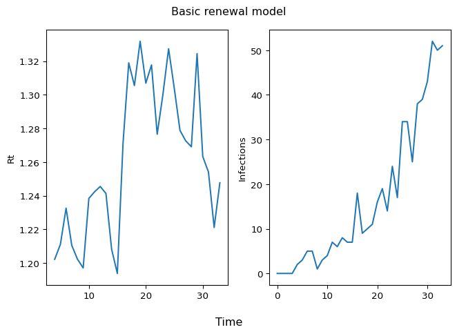
To understand what has been accomplished here, visualize an \(R_t\) sample path (left panel) and infections over time (right panel):

import matplotlib.pyplot as plt

fig, axs = plt.subplots(1, 2)

# Rt plot
axs[0].plot(sim_data.Rt)
axs[0].set_ylabel("Rt")

# Infections plot
axs[1].plot(sim_data.observed_infections)
axs[1].set_ylabel("Infections")

fig.suptitle("Basic renewal model")
fig.supxlabel("Time")
plt.tight_layout()
plt.show()

To fit the model, we can use the run() method of the RtInfectionsRenewalModel class (an inherited method from the metaclass Model). model1.run() will call the run method of the model1 object, which will generate an instance of model MCMC simulation, with 2000 warm-up iterations for the MCMC algorithm, used to tune the parameters of the MCMC algorithm to improve efficiency of the sampling process. From the posterior distribution of the model parameters, 1000 samples will be drawn and used to estimate the posterior distributions and compute summary statistics. Observed data is provided to the model using the sim_data object previously generated. mcmc_args provides additional arguments for the MCMC algorithm.

import jax

model1.run(
    num_warmup=2000,
    num_samples=1000,
    data_observed_infections=sim_data.observed_infections,
    rng_key=jax.random.PRNGKey(54),
    mcmc_args=dict(progress_bar=False, num_chains=2),
)

/home/runner/work/multisignal-epi-inference/multisignal-epi-inference/model/src/pyrenew/metaclass.py:304: UserWarning: There are not enough devices to run parallel chains: expected 2 but got 1. Chains will be drawn sequentially. If you are running MCMC in CPU, consider using `numpyro.set_host_device_count(2)` at the beginning of your program. You can double-check how many devices are available in your system using `jax.local_device_count()`.
  self.mcmc = MCMC(

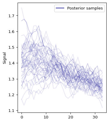
Now, let’s investigate the output, particularly the posterior distribution of the \(R_t\) estimates:

out = model1.plot_posterior(var="Rt")

We can use ArviZ package to create model diagnostics and visualizations. We start by converting the fitted model to ArviZ InferenceData object:

import arviz as az

idata = az.from_numpyro(model1.mcmc)

and use the InferenceData to compute the model-fit diagnostics. Here, we show diagnostic summary for the first 10 effective reproduction number \(R_t\).

diagnostic_stats_summary = az.summary(
    idata.posterior["Rt"],
    kind="diagnostics",
)

print(diagnostic_stats_summary[:10])

       mcse_mean  mcse_sd  ess_bulk  ess_tail  r_hat
Rt[0]      0.003    0.002    1309.0    1339.0    1.0
Rt[1]      0.003    0.002    1331.0    1264.0    1.0
Rt[2]      0.003    0.002    1340.0    1395.0    1.0
Rt[3]      0.003    0.002    1421.0    1335.0    1.0
Rt[4]      0.002    0.002    1459.0    1464.0    1.0
Rt[5]      0.002    0.002    1597.0    1303.0    1.0
Rt[6]      0.002    0.002    1539.0    1454.0    1.0
Rt[7]      0.002    0.001    1707.0    1529.0    1.0
Rt[8]      0.002    0.001    1494.0    1674.0    1.0
Rt[9]      0.002    0.001    1951.0    1517.0    1.0

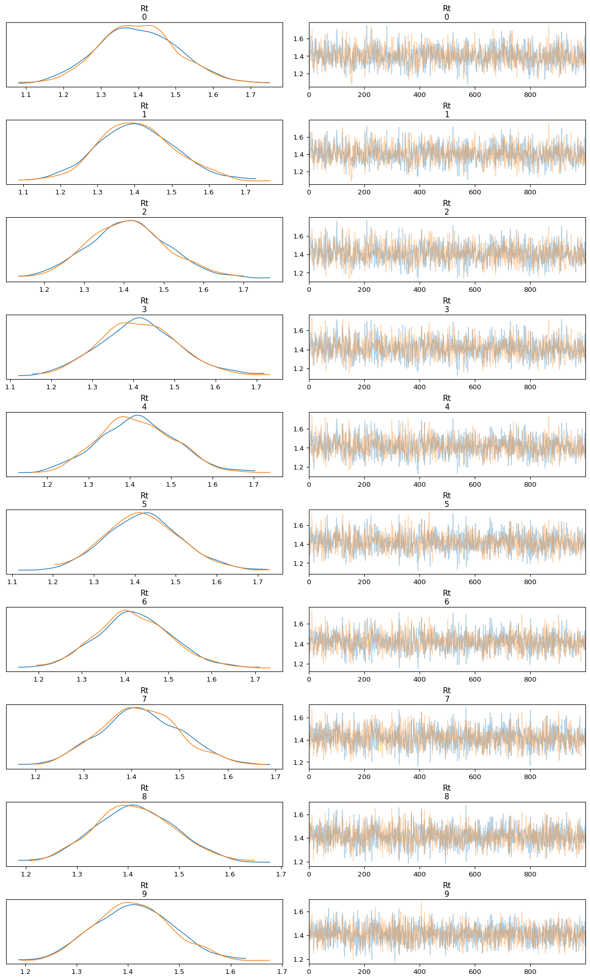
Below we use plot_trace to inspect the trace of the first 10 \(R_t\) estimates.

plt.rcParams["figure.constrained_layout.use"] = True

az.plot_trace(
    idata.posterior,
    var_names=["Rt"],
    coords={"Rt_dim_0": np.arange(10)},
    compact=False,
);

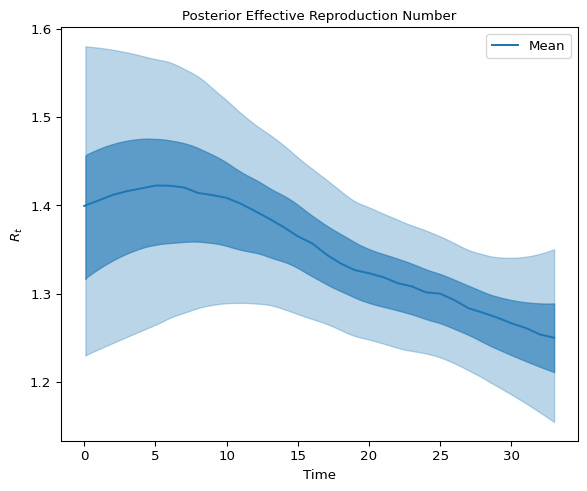
We inspect the posterior distribution of \(R_t\) by plotting the 90% and 50% highest density intervals:

x_data = idata.posterior["Rt_dim_0"]
y_data = idata.posterior["Rt"]

fig, axes = plt.subplots(figsize=(6, 5))
az.plot_hdi(
    x_data,
    y_data,
    hdi_prob=0.9,
    color="C0",
    fill_kwargs={"alpha": 0.3},
    ax=axes,
)

az.plot_hdi(
    x_data,
    y_data,
    hdi_prob=0.5,
    color="C0",
    fill_kwargs={"alpha": 0.6},
    ax=axes,
)

# Add mean of the posterior to the figure
mean_Rt = np.mean(idata.posterior["Rt"], axis=1)
axes.plot(x_data, mean_Rt[0], color="C0", label="Mean")
axes.legend()
axes.set_title("Posterior Effective Reproduction Number", fontsize=10)
axes.set_xlabel("Time", fontsize=10)
axes.set_ylabel("$R_t$", fontsize=10);

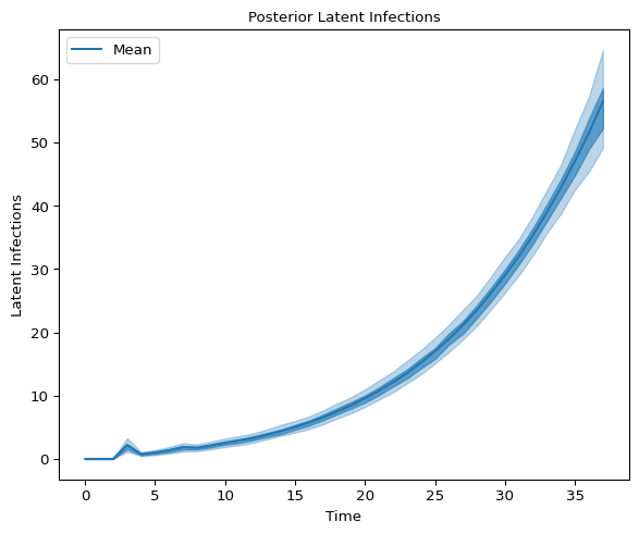
and latent infections:

x_data = idata.posterior["all_latent_infections_dim_0"]
y_data = idata.posterior["all_latent_infections"]

fig, axes = plt.subplots(figsize=(6, 5))
az.plot_hdi(
    x_data,
    y_data,
    hdi_prob=0.9,
    color="C0",
    smooth=False,
    fill_kwargs={"alpha": 0.3},
    ax=axes,
)

az.plot_hdi(
    x_data,
    y_data,
    hdi_prob=0.5,
    color="C0",
    smooth=False,
    fill_kwargs={"alpha": 0.6},
    ax=axes,
)

# Add mean of the posterior to the figure
mean_latent_infection = np.mean(
    idata.posterior["all_latent_infections"], axis=1
)
axes.plot(x_data, mean_latent_infection[0], color="C0", label="Mean")
axes.legend()
axes.set_title("Posterior Latent Infections", fontsize=10)
axes.set_xlabel("Time", fontsize=10)
axes.set_ylabel("Latent Infections", fontsize=10);

Architecture of pyrenew#

pyrenew leverages numpyro’s flexibility to build models via composition. As a principle, most objects in pyrenew can be treated as random variables we can sample. At the top-level pyrenew has two metaclasses from which most objects inherit: RandomVariable and Model. From them, the following four sub-modules arise:

The process sub-module,
The deterministic sub-module,
The observation sub-module,
The latent sub-module, and
The models sub-module

The first four are collections of instances of RandomVariable, and the last is a collection of instances of Model. The following diagram shows a detailed view of how metaclasses, modules, and classes interact to create the RtInfectionsRenewalModel instantiated in the previous section:

Getting started with pyrenew

Contents

Getting started with pyrenew#

The fundamentals#

‘Hello world’ model#

Architecture of pyrenew#