Fitting a Hospital Admissions-only Model#
This document illustrates how a hospital admissions-only model can be fitted using data from the Pyrenew package, particularly the wastewater dataset. The CFA wastewater team created this dataset, which contains simulated data.
Model definition#
In this section, we provide the formal definition of the model. The hospitalization model is a semi-mechanistic model that describes the number of observed hospital admissions as a function of a set of latent variables. Mainly, the observed number of hospital admissions is discretely distributed with location at the number of latent hospital admissions:
Where \(h(t)\) is the observed number of hospital admissions at time \(t\), and \(H(t)\) is the number of latent hospital admissions at time \(t\). The distribution \(\text{HospDist}\) is discrete. For this example, we will use a negative binomial distribution:
Were \(d(\tau)\) is the infection to hospitalization interval,
\(I(t)\) is the number of latent infections at time \(t\),
\(p_\mathrm{hosp}(t)\) is the infection to hospitalization rate, and
\(\omega(t)\) is the day-of-the-week effect at time \(t\); the
last section provides an example building such a RandomVariable.
The number of latent hospital admissions at time \(t\) is a function of the number of latent infections at time \(t\) and the infection to hospitalization rate. The latent infections are modeled as a renewal process:
The reproductive number \(R(t)\) is modeled as a random walk process:
Data processing#
We start by loading the data and inspecting the first five rows.
import polars as pl
from pyrenew import datasets

dat = datasets.load_wastewater()
dat.head(5)
t |
lab _wwtp _uniq ue_id |
log _conc |
date |
lod_s ewage |
belo w_lod |
da ily_h osp_a dmits |
pop |
for ecast _date |
h osp_c alibr ation _time |
site |
w w_pop |
inf_ per_c apita |
|
|---|---|---|---|---|---|---|---|---|---|---|---|---|---|
i64 |
i64 |
f64 |
date |
f64 |
i64 |
i64 |
i64 |
f64 |
date |
i64 |
i64 |
f64 |
f64 |
1 |
1 |
null |
2023- 10-30 |
null |
null |
6 |
6 |
1e6 |
2024- 02-05 |
90 |
1 |
400 000.0 |
0.0 00663 |
1 |
2 |
null |
2023- 10-30 |
null |
null |
6 |
6 |
1e6 |
2024- 02-05 |
90 |
1 |
400 000.0 |
0.0 00663 |
1 |
3 |
null |
2023- 10-30 |
null |
null |
6 |
6 |
1e6 |
2024- 02-05 |
90 |
2 |
200 000.0 |
0.0 00663 |
1 |
4 |
null |
2023- 10-30 |
null |
null |
6 |
6 |
1e6 |
2024- 02-05 |
90 |
3 |
100 000.0 |
0.0 00663 |
1 |
5 |
null |
2023- 10-30 |
null |
null |
6 |
6 |
1e6 |
2024- 02-05 |
90 |
4 |
50 000.0 |
0.0 00663 |
The data shows one entry per site, but the way it was simulated, the number of admissions is the same across sites. Thus, we will only keep the first observation per day.
# Keeping the first observation of each date
dat = dat.group_by("date").first().select(["date", "daily_hosp_admits"])

# Now, sorting by date
dat = dat.sort("date")

# Keeping the first 90 days
dat = dat.head(90)

dat.head(5)
date |
daily_hosp_admits |
|---|---|
date |
i64 |
2023-10-30 |
6 |
2023-10-31 |
8 |
2023-11-01 |
4 |
2023-11-02 |
8 |
2023-11-03 |
4 |
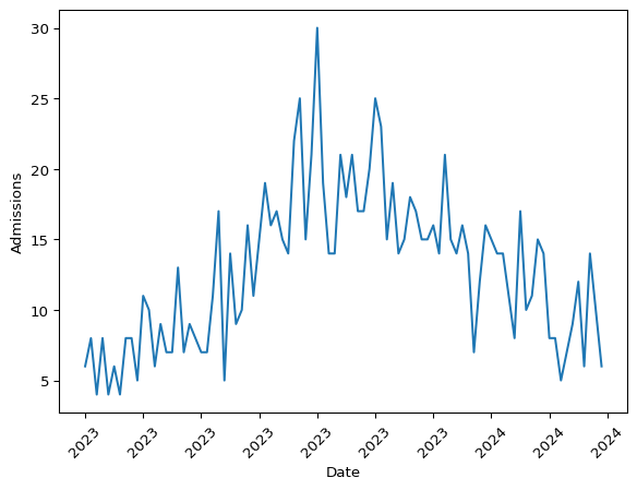
Let’s take a look at the daily prevalence of hospital admissions.
import matplotlib.pyplot as plt

# Rotating the x-axis labels, and only showing ~10 labels
ax = plt.gca()
ax.xaxis.set_major_locator(plt.MaxNLocator(nbins=10))
ax.xaxis.set_tick_params(rotation=45)
plt.plot(dat["date"].to_numpy(), dat["daily_hosp_admits"].to_numpy())
plt.xlabel("Date")
plt.ylabel("Admissions")
plt.show()
Building the model#
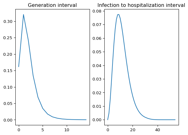
First, we will extract two datasets we will use as deterministic quantities: the generation interval and the infection to hospitalization interval.
gen_int = datasets.load_generation_interval()
inf_hosp_int = datasets.load_infection_admission_interval()

# We only need the probability_mass column of each dataset
gen_int_array = gen_int["probability_mass"].to_numpy()
gen_int = gen_int_array
inf_hosp_int = inf_hosp_int["probability_mass"].to_numpy()

# Taking a pick at the first 5 elements of each
gen_int[:5], inf_hosp_int[:5]

# Visualizing both quantities side by side
fig, axs = plt.subplots(1, 2)

axs[0].plot(gen_int)
axs[0].set_title("Generation interval")
axs[1].plot(inf_hosp_int)
axs[1].set_title("Infection to hospitalization interval")
plt.show()
With these two in hand, we can start building the model. First, we will define the latent hospital admissions:
from pyrenew import latent, deterministic, metaclass
import jax.numpy as jnp
import numpyro.distributions as dist

inf_hosp_int = deterministic.DeterministicPMF(
    inf_hosp_int, name="inf_hosp_int"
)

hosp_rate = metaclass.DistributionalRV(
    dist=dist.LogNormal(jnp.log(0.05), 0.1),
    name="IHR",
)

latent_hosp = latent.HospitalAdmissions(
    infection_to_admission_interval_rv=inf_hosp_int,
    infect_hosp_rate_rv=hosp_rate,
)
/home/runner/.cache/pypoetry/virtualenvs/pyrenew-ay_vsbmF-py3.12/lib/python3.12/site-packages/tqdm/auto.py:21: TqdmWarning: IProgress not found. Please update jupyter and ipywidgets. See https://ipywidgets.readthedocs.io/en/stable/user_install.html
  from .autonotebook import tqdm as notebook_tqdm
The inf_hosp_int is a DeterministicPMF object that takes the
infection to hospitalization interval as input. The hosp_rate is a
DistributionalRV object that takes a numpyro distribution to
represent the infection to hospitalization rate. The
HospitalAdmissions class is a RandomVariable that takes two
distributions as inputs: the infection to admission interval and the
infection to hospitalization rate. Now, we can define the rest of the
other components:
from pyrenew import model, process, observation, metaclass, transformation
from pyrenew.latent import InfectionSeedingProcess, SeedInfectionsExponential

# Infection process
latent_inf = latent.Infections()
I0 = InfectionSeedingProcess(
    "I0_seeding",
    metaclass.DistributionalRV(
        dist=dist.LogNormal(loc=jnp.log(100), scale=0.5), name="I0"
    ),
    SeedInfectionsExponential(
        gen_int_array.size,
        deterministic.DeterministicVariable(0.5, name="rate"),
    ),
)

# Generation interval and Rt
gen_int = deterministic.DeterministicPMF(gen_int, name="gen_int")
rtproc = process.RtRandomWalkProcess(
    Rt0_dist=dist.TruncatedNormal(loc=1.2, scale=0.2, low=0),
    Rt_transform=transformation.ExpTransform().inv,
    Rt_rw_dist=dist.Normal(0, 0.025),
)

# The observation model
obs = observation.NegativeBinomialObservation(concentration_prior=1.0)
Notice all the components are RandomVariable instances. We can now
build the model:
hosp_model = model.HospitalAdmissionsModel(
    latent_infections_rv=latent_inf,
    latent_hosp_admissions_rv=latent_hosp,
    I0_rv=I0,
    gen_int_rv=gen_int,
    Rt_process_rv=rtproc,
    hosp_admission_obs_process_rv=obs,
)
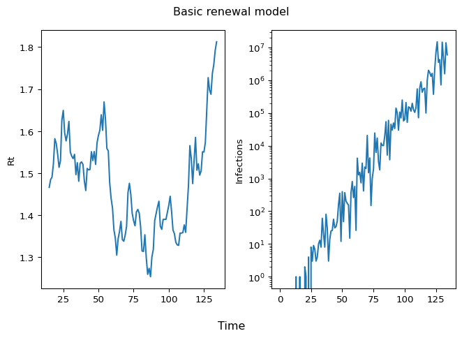
Let’s simulate to check if the model is working:
import numpyro as npro
import numpy as np

timeframe = 120

np.random.seed(223)
with npro.handlers.seed(rng_seed=np.random.randint(1, timeframe)):
    sim_data = hosp_model.sample(n_timepoints_to_simulate=timeframe)
/home/runner/.cache/pypoetry/virtualenvs/pyrenew-ay_vsbmF-py3.12/lib/python3.12/site-packages/jax/_src/numpy/lax_numpy.py:3044: FutureWarning: None encountered in jnp.array(); this is currently treated as NaN. In the future this will result in an error.
  return array(arys[0], copy=False, ndmin=1)
import matplotlib.pyplot as plt

fig, axs = plt.subplots(1, 2)

# Rt plot
axs[0].plot(sim_data.Rt)
axs[0].set_ylabel("Rt")

# Infections plot
axs[1].plot(sim_data.observed_hosp_admissions)
axs[1].set_ylabel("Infections")
axs[1].set_yscale("log")

fig.suptitle("Basic renewal model")
fig.supxlabel("Time")
plt.tight_layout()
plt.show()
Fitting the model#
We can fit the model to the data. We will use the run method of the
model object:
import jax

hosp_model.run(
    num_samples=2000,
    num_warmup=2000,
    data_observed_hosp_admissions=dat["daily_hosp_admits"].to_numpy(),
    rng_key=jax.random.PRNGKey(54),
    mcmc_args=dict(progress_bar=False, num_chains=2),
)
/home/runner/work/multisignal-epi-inference/multisignal-epi-inference/model/src/pyrenew/metaclass.py:304: UserWarning: There are not enough devices to run parallel chains: expected 2 but got 1. Chains will be drawn sequentially. If you are running MCMC in CPU, consider using `numpyro.set_host_device_count(2)` at the beginning of your program. You can double-check how many devices are available in your system using `jax.local_device_count()`.
  self.mcmc = MCMC(
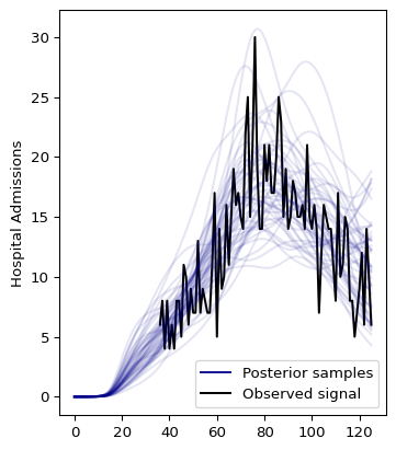
We can use the plot_posterior method to visualize the results [1]:
out = hosp_model.plot_posterior(
    var="latent_hospital_admissions",
    ylab="Hospital Admissions",
    obs_signal=np.pad(
        dat["daily_hosp_admits"].to_numpy().astype(float),
        (gen_int_array.size, 0),
        constant_values=np.nan,
    ),
)
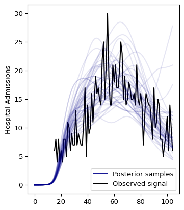
The first half of the model is not looking good. The reason is that the infection to hospitalization interval PMF makes it unlikely to observe admissions from the beginning. The following section shows how to fix this.
Padding the model#
We can use the padding argument to solve the overestimation of hospital
admissions in the first half of the model. By setting padding > 0,
the model then assumes that the first padding observations are
missing; thus, only observations after padding will count towards
the likelihood of the model. In practice, the model will extend the
estimated Rt and latent infections by padding days, given time to
adjust to the observed data. The following code will add 21 days of
missing data at the beginning of the model and re-estimate it with
padding = 21:
days_to_impute = 21

# Add 21 Nas to the beginning of dat_w_padding
dat_w_padding = np.pad(
    dat["daily_hosp_admits"].to_numpy().astype(float),
    (days_to_impute, 0),
    constant_values=np.nan,
)


hosp_model.run(
    num_samples=2000,
    num_warmup=2000,
    data_observed_hosp_admissions=dat_w_padding,
    rng_key=jax.random.PRNGKey(54),
    mcmc_args=dict(progress_bar=False, num_chains=2),
    padding=days_to_impute,  # Padding the model
)
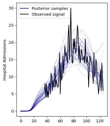
And plotting the results:
out = hosp_model.plot_posterior(
    var="latent_hospital_admissions",
    ylab="Hospital Admissions",
    obs_signal=np.pad(
        dat_w_padding, (gen_int_array.size, 0), constant_values=np.nan
    ),
)
We can use ArviZ to visualize the results. Let’s start by converting the fitted model to Arviz InferenceData object:
import arviz as az

idata = az.from_numpyro(hosp_model.mcmc)
We obtain the summary of model diagnostics and print the diagnostics for
latent_hospital_admissions[1]
diagnostic_stats_summary = az.summary(
    idata.posterior,
    kind="diagnostics",
)

print(diagnostic_stats_summary.loc["latent_hospital_admissions[1]"])
mcse_mean       0.0
mcse_sd         0.0
ess_bulk     5000.0
ess_tail     2788.0
r_hat           1.0
Name: latent_hospital_admissions[1], dtype: float64
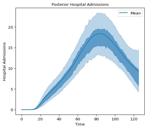
Below we plot 90% and 50% highest density intervals for latent hospital admissions using plot_hdi:
x_data = idata.posterior["latent_hospital_admissions_dim_0"]
y_data = idata.posterior["latent_hospital_admissions"]

fig, axes = plt.subplots(figsize=(6, 5))
az.plot_hdi(
    x_data,
    y_data,
    hdi_prob=0.9,
    color="C0",
    smooth=False,
    fill_kwargs={"alpha": 0.3},
    ax=axes,
)

az.plot_hdi(
    x_data,
    y_data,
    hdi_prob=0.5,
    color="C0",
    smooth=False,
    fill_kwargs={"alpha": 0.6},
    ax=axes,
)

# Add mean of the posterior to the figure
mean_latent_hosp_admission = np.mean(
    idata.posterior["latent_hospital_admissions"], axis=1
)
axes.plot(x_data, mean_latent_hosp_admission[0], color="C0", label="Mean")
axes.legend()
axes.set_title("Posterior Hospital Admissions", fontsize=10)
axes.set_xlabel("Time", fontsize=10)
axes.set_ylabel("Hospital Admissions", fontsize=10);
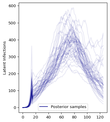
We can also take a look at the latent infections:
out2 = hosp_model.plot_posterior(
    var="all_latent_infections", ylab="Latent Infections"
)
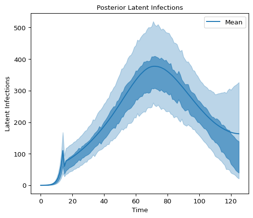
and the distribution of latent infections
x_data = idata.posterior["all_latent_infections_dim_0"]
y_data = idata.posterior["all_latent_infections"]

fig, axes = plt.subplots(figsize=(6, 5))
az.plot_hdi(
    x_data,
    y_data,
    hdi_prob=0.9,
    color="C0",
    smooth=False,
    fill_kwargs={"alpha": 0.3},
    ax=axes,
)

az.plot_hdi(
    x_data,
    y_data,
    hdi_prob=0.5,
    color="C0",
    smooth=False,
    fill_kwargs={"alpha": 0.6},
    ax=axes,
)

# Add mean of the posterior to the figure
mean_latent_infection = np.mean(
    idata.posterior["all_latent_infections"], axis=1
)
axes.plot(x_data, mean_latent_infection[0], color="C0", label="Mean")
axes.legend()
axes.set_title("Posterior Latent Infections", fontsize=10)
axes.set_xlabel("Time", fontsize=10)
axes.set_ylabel("Latent Infections", fontsize=10);
Round 2: Incorporating day-of-the-week effects#
We will re-use the infection to admission interval and infection to
hospitalization rate from the previous model. But we will also add a
day-of-the-week effect distribution. To do this, we will create a new
instance of RandomVariable to model the effect. The class will be
based on a truncated normal distribution with a mean of 1.0 and a
standard deviation of 0.5. The distribution will be truncated between
0.1 and 10.0. The random variable will be repeated for the number of
weeks in the dataset. Note a similar weekday effect is implemented in
its own module, with example code here.
from pyrenew import metaclass
import numpyro as npro


class DayOfWeekEffect(metaclass.RandomVariable):
    """Day of the week effect"""

    def __init__(self, len: int):
        """Initialize the day of the week effect distribution
        Parameters
        ----------
        len : int
            The number of observations
        """
        self.nweeks = int(jnp.ceil(len / 7))
        self.len = len

    @staticmethod
    def validate():
        return None

    def sample(self, **kwargs):
        ans = npro.sample(
            name="dayofweek_effect",
            fn=npro.distributions.TruncatedNormal(
                loc=1.0, scale=0.5, low=0.1, high=10.0
            ),
            sample_shape=(7,),
        )

        return jnp.tile(ans, self.nweeks)[: self.len]


# Initializing the RV
dayofweek_effect = DayOfWeekEffect(dat.shape[0])
Notice that the instance’s nweeks and len members are passed
during construction. Trying to compute the number of weeks and the
length of the dataset in the validate method will raise a jit
error in jax as the shape and size of elements are not known during
the validation step, which happens before the model is run. With the new
effect, we can rebuild the latent hospitalization model:
latent_hosp_wday_effect = latent.HospitalAdmissions(
    infection_to_admission_interval_rv=inf_hosp_int,
    infect_hosp_rate_rv=hosp_rate,
    day_of_week_effect_rv=dayofweek_effect,
)

hosp_model_weekday = model.HospitalAdmissionsModel(
    latent_infections_rv=latent_inf,
    latent_hosp_admissions_rv=latent_hosp_wday_effect,
    I0_rv=I0,
    gen_int_rv=gen_int,
    Rt_process_rv=rtproc,
    hosp_admission_obs_process_rv=obs,
)
Running the model (with the same padding as before):
hosp_model_weekday.run(
    num_samples=2000,
    num_warmup=2000,
    data_observed_hosp_admissions=dat_w_padding,
    rng_key=jax.random.PRNGKey(54),
    mcmc_args=dict(progress_bar=False),
    padding=days_to_impute,
)
And plotting the results:
out = hosp_model_weekday.plot_posterior(
    var="latent_hospital_admissions",
    ylab="Hospital Admissions",
    obs_signal=np.pad(
        dat_w_padding, (gen_int_array.size, 0), constant_values=np.nan
    ),
)