RtGam is an R package for real-time estimation of epidemic growth rates. The package fits a smooth trend over time to an epidemic timeseries with a generalized additive model (GAM). From this fitted trend, it generates a short-term forecast and estimates the time-varying effective reproductive number, \(R_t\) and intrinsic growth rate, \(r\).
This vignette gives a brief overview of RtGam. It walks through how to fit a model to an epidemic timeseries and interpret the results.
Setup
This vignette assumes you have the RtGam package installed and
loaded. This vignette uses ggplot2.
Data
The RtGam package requires a time series of observed
incident case counts. For demonstration purposes, the package includes a
simulated epidemic dataset, stochastic_sir_rt, adapted from
Gostic et al. (2020).
In this example dataset, obs_cases is the vector of
observed case counts, and reference_date is the
corresponding vector of dates. The dataset has a timeseries of 299 days
that we’ll subset to 60 days to make plotting easier.
data <- stochastic_sir_rt[41:100, ]
ggplot(data) +
  geom_point(aes(reference_date, obs_cases)) +
  theme_bw() +
  labs(x = "Reference date", y = "Observed cases")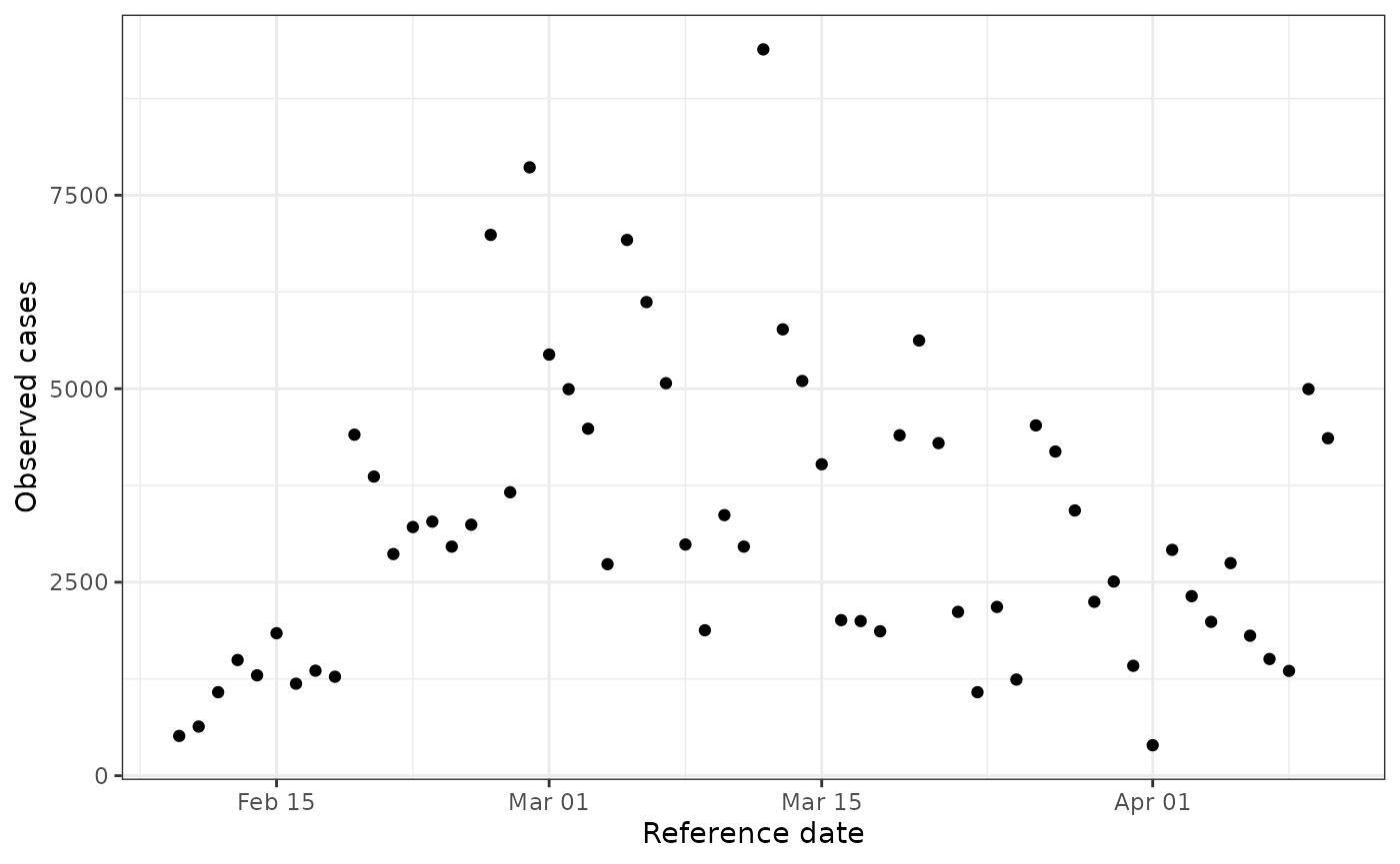
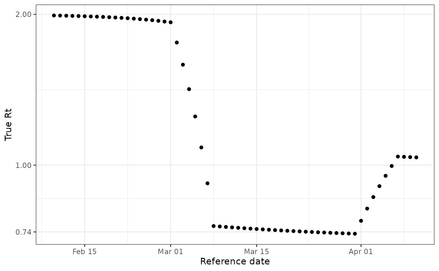
Because this dataset was simulated, we know the true \(R_t\) that generated the epidemic timeseries.
ggplot(data) +
  geom_point(aes(reference_date, true_rt)) +
  theme_bw() +
  labs(x = "Reference date", y = "True Rt") +
  scale_y_continuous(
    trans = "log",
    labels = scales::number_format(accuracy = 0.01)
  )
For more on this dataset see ?stochastic_sir_rt.
Fitting the Model
To fit an RtGam model, provide a vector of observed case
counts and their corresponding dates. The model can automatically select
hyperparameters like the smoothing basis dimension and the penalty basis
dimension.
fit <- RtGam(
  cases = data[["obs_cases"]],
  reference_date = data[["reference_date"]]
)
print(fit)
#> ===============================
#> Fitted RtGam model object (gam)
#> ===============================
#>
#> Model type: Adaptive (m = 2)
#> Specified maximum smoothing basis dimension: 27
#> Family: Negative Binomial(12.448)
#> Link function: log
#> Using day-of-week effects
#> ===============================
#>
#> Observed data points: 60
#> Distinct reference dates: 60
#> Distinct groups: 1
#> Day-of-week levels: 7
To select your own smoothing or penalty basis dimension you can
provide those parameters to the model. The penalty basis dimension can
be specified with the k argument and the smooth basis
dimension can be specified with the m argument. For
example, we can decrease the penalty basis dimension of the model by
setting m to 1. See smooth_dim_heuristic() and
penalty_dim_heuristic() for more on how these basis
dimensions are set and when to change them.
fit_non_adaptive <- RtGam(
  cases = data[["obs_cases"]],
  reference_date = data[["reference_date"]],
  m = 1
)
print(fit_non_adaptive)
#> ===============================
#> Fitted RtGam model object (gam)
#> ===============================
#>
#> Model type: Non-adaptive (m = 1)
#> Specified maximum smoothing basis dimension: 27
#> Family: Negative Binomial(12.707)
#> Link function: log
#> Using day-of-week effects
#> ===============================
#>
#> Observed data points: 60
#> Distinct reference dates: 60
#> Distinct groups: 1
#> Day-of-week levels: 7
Note that RtGam throws warnings if diagnostic issues are detected.
See ?RtGam for more details on how to specify a model and
?check_diagnostics for more on model diagnostics.
Analyzing Results
Posterior predicted cases
The predict() method draws samples from the posterior
distribution of the fitted model. By default it draws 100 sampled
timeseries of posterior predicted cases.
head(predict(fit))
#>   reference_date .response .draw
#> 1     2023-02-10       700     1
#> 2     2023-02-10       505    86
#> 3     2023-02-10      1000    84
#> 4     2023-02-10       460    82
#> 5     2023-02-10       400    80
#> 6     2023-02-10       428    24
Calling plot on the fitted model object also draws
posterior samples and plots them against the provided timeseries of
cases.
plot(fit)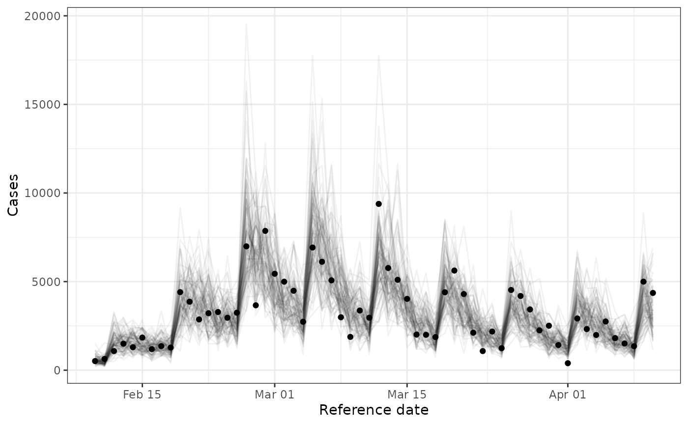
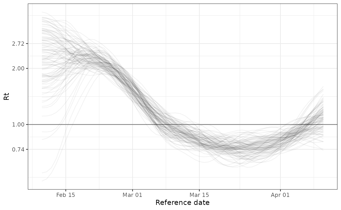
Expected \(R_t\)
Producing an estimate of \(R_t\)
requires some additional information. It needs the
mean_delay, which is the expected number of days from a
case’s infection to the case being counted. For example in a
timeseries of hospitalizations, it’s the average number of days between
infection and being hospitalized.
It also requires an estimate of the generation interval, which can be
drawn from the literature or estimated separately using data on paired
cases. RtGam expects the GI to be formatted as a
probability mass function. We recommend using the package primarycensored to
format a known generation interval distribution as a PMF. The
probability mass function should have the first element dropped and
replaced with a 0 because the underlying renewal-equation based approach
assumes no same-day transmission.
In this simulated example, cases are observed immediately so the mean
delay is 0. We have pre-generated the generation interval probability
mass function (see more with ?sir_gt_pmf).
plot(
  fit,
  parameter = "Rt",
  mean_delay = 0,
  gi_pmf = sir_gt_pmf
)
Model validation
Comparing the posterior draws from the fitted model posterior to the simulated ground truth suggests that the model is able to recover \(R_t\) from this timeseries. The model is able to identify and correctly time the sharp drop in \(R_t\) in early March and the rise in \(R_t\) in early April. However, we can see that the model has high uncertainty during initialization and oversmooths the sharp decline in early March.
plot(
  fit,
  parameter = "Rt",
  mean_delay = 0,
  gi_pmf = sir_gt_pmf
) +
  geom_point(aes(reference_date, true_rt), data = data)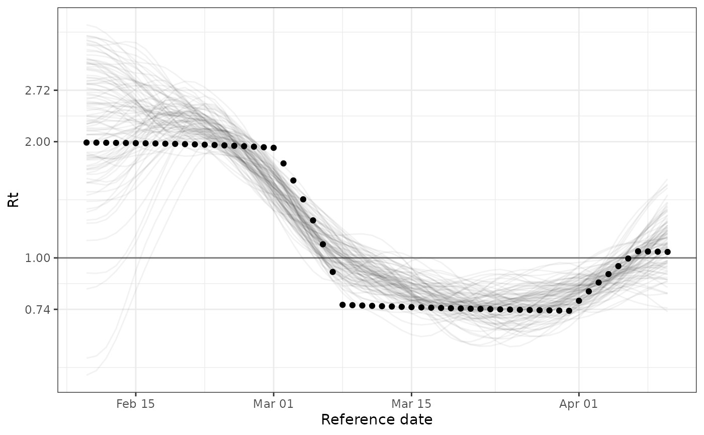
Future development effort will aim to improve model performance on challenging datasets like this example.
Additional Resources
To provide feedback or ask questions, refer to the package’s GitHub repository.
Note: This package is in early development. Outputs may be misleading or incorrect. Use with caution and refer to the repository for updates.