Wastewater informed forecasting: fit to simulated data

This vignette steps through the pre-processing and fitting procedure to forecast state-level hospital admissions using simulated data. The code can be adapted for your own datasets by replacing the joined hospital admissions + site-lab level wastewater dataset, here called, example_df, with your own dataset and varying the parameters that are pre-specified. See the documentation for example_df to format your data in a similar manner. For an example of how to do this from the raw generated outputs, see the generate_simulated_data.R function. Note that if using real data, the part about comparing the inferred parameters to the known truth parameters will not be relevant as this information will not be available.

Rationale

Load the data

# Example of how to generate new simulated data with user-specified parameters
# by calling `generate_simulated_data()`
# See function documentation to modify R(t), number of sites, etc.
example_df <- cfaforecastrenewalww::example_df

The generate_simulated_data.R file can be used to generate this simulated data where individual sites exhibit their own site-level infection dynamics. Setting n_sites to one allows the user to generate data amenable to the state-level aggregated wastewater model, or alternatively, site-level data can be generated and then aggregated using population weighted averaging of the concentration to generate a single state-level wastewater data stream. However, this vignette assumes you have wastewater data from one or more sites that represent some subset of the population for which you have hospital admissions data for.

Data exploration

The example dataframe is a long tidy data frame with hospital admissions alongside site-level wastewater data, corresponding to a single observation for each lab-site-day. We assign an arbitrary date to the time series so that we can assign a week day to each day. We additionally include a column containing the daily hospital admissions through the forecast period daily_hosp_admits_for_eval. This will be used for evaluating our simulated data inference procedure. See documentation of example_df for a full description of each column.

head(example_df)

## # A tibble: 6 × 14
##       t lab_wwtp_unique_id log_conc date       lod_sewage below_LOD
##   <int>              <int>    <dbl> <date>          <dbl>     <dbl>
## 1     1                  1       NA 2023-10-30         NA        NA
## 2     1                  2       NA 2023-10-30         NA        NA
## 3     1                  3       NA 2023-10-30         NA        NA
## 4     1                  4       NA 2023-10-30         NA        NA
## 5     1                  5       NA 2023-10-30         NA        NA
## 6     2                  1       NA 2023-10-31         NA        NA
## # ℹ 8 more variables: daily_hosp_admits <dbl>,
## #   daily_hosp_admits_for_eval <dbl>, pop <dbl>, forecast_date <date>,
## #   hosp_calibration_time <dbl>, site <dbl>, ww_pop <dbl>, inf_per_capita <dbl>

Make some plots of the hospital admissions and wastewater data

The model will jointly calibrate to state-level hospital admissions and the site-level wastewater data. It will estimate underlying latent incident infection curves, either for each site coming from a shared distribution with a global mean of the state-level incident infection curve, or it will estimate a single state-level incident infection curve that is assumes to be homogenous across all sites. From the simulated data, we impose a delay from the date of the forecast to the last observed hospital admissions, to reflect the current data reporting structure in the US. We also include variable reporting frequency and latency in the site-level wastewater data, to reflect the real heterogeneity we observe in the NWSS data in real-time.

ggplot(example_df) +
  geom_point(
    aes(
      x = date, y = exp(log_conc),
      color = as.factor(lab_wwtp_unique_id)
    ),
    show.legend = FALSE
  ) +
  geom_point(
    data = example_df %>% filter(below_LOD == 1),
    aes(x = date, y = exp(log_conc), color = "red"),
    show.legend = FALSE
  ) +
  geom_hline(aes(yintercept = exp(lod_sewage)), linetype = "dashed") +
  facet_wrap(~lab_wwtp_unique_id, scales = "free") +
  geom_vline(aes(xintercept = forecast_date), linetype = "dashed") +
  xlab("") +
  ylab("Genome copies/mL") +
  ggtitle("Lab-site level wastewater concentration") +
  theme_bw()

## Warning: Removed 568 rows containing missing values or values outside the scale range
## (`geom_point()`).

## Warning: Removed 568 rows containing missing values or values outside the scale range
## (`geom_hline()`).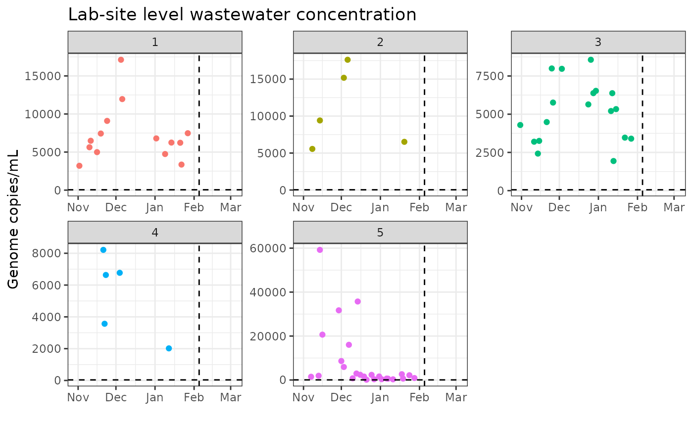

ggplot(example_df) +
  geom_point(aes(x = date, y = daily_hosp_admits_for_eval),
    shape = 21, color = "black", fill = "white"
  ) +
  geom_point(aes(x = date, y = daily_hosp_admits)) +
  geom_vline(aes(xintercept = forecast_date), linetype = "dashed") +
  xlab("") +
  ylab("Daily hospital admissions") +
  ggtitle("State level hospital admissions") +
  theme_bw()

## Warning: Removed 185 rows containing missing values or values outside the scale range
## (`geom_point()`).

Format data for inference in stan

The model expects input data in a certain format. The cfaforecastrenewalww R package provides helper functions to facilitate preparing data for ingestion by the model.

Hyperparameters for prior distributions and other fixed quantites should be specified in a .toml file, which the function get_params() reads and validates. We have provided an example parameter file, example_params.toml, with the package.

We’ll read it in and examine it here:

params <- get_params(
  system.file("extdata", "example_params.toml",
    package = "cfaforecastrenewalww"
  )
)
params

##   backward_scale backward_shape gt_max   mu_gi neg_binom_mu neg_binom_size    r
## 1            3.6            1.5     15 0.92877      6.98665       2.490848 0.15
##   sigma_gi uot autoreg_p_hosp_a autoreg_p_hosp_b autoreg_rt_a autoreg_rt_b
## 1    0.526  50                1              100            2           40
##   autoreg_rt_site_a autoreg_rt_site_b dur_inf eta_sd_sd i0_certainty
## 1                 1                 4       7      0.01            5
##   infection_feedback_prior_logmean infection_feedback_prior_logsd
## 1                          6.37408                            0.4
##   initial_growth_prior_mean initial_growth_prior_sd r_prior_mean r_prior_sd
## 1                         0                    0.01            1          1
##   sigma_i0_prior_mode sigma_i0_prior_sd sigma_rt_prior inv_sqrt_phi_prior_mean
## 1                   0               0.5            0.1                     0.1
##   inv_sqrt_phi_prior_sd p_hosp_mean p_hosp_sd_logit p_hosp_w_sd_sd
## 1             0.1414214        0.01             0.3           0.01
##   wday_effect_prior_mean wday_effect_prior_sd duration_shedding_mean
## 1              0.1428571                 0.05                     17
##   duration_shedding_sd log10_g_prior_mean log10_g_prior_sd log_g_prior_mean
## 1                    3                 12                2         27.63102
##   log_g_prior_sd log_phi_g_prior_mean log_phi_g_prior_sd
## 1        4.60517            -2.302585                  5
##   ml_of_ww_per_person_day sigma_ww_site_prior_mean_mean
## 1                  227000                             1
##   sigma_ww_site_prior_mean_sd sigma_ww_site_prior_sd_mean
## 1                           1                           0
##   sigma_ww_site_prior_sd_sd t_peak_mean t_peak_sd viral_peak_mean viral_peak_sd
## 1                         1           5         1             5.1           0.5
##   ww_site_mod_sd_sd
## 1              0.25

The example values in example_params.toml are the same as those stored in cfaforecastrenewalww::param_df and used (via prior predictive simulation to generate the simulated data in cfaforecastrenewalww::example_df.

forecast_date <- example_df %>%
  pull(forecast_date) %>%
  unique()
forecast_time <- as.integer(max(example_df$date) - forecast_date)

# Assign the model that we want to fit to  so that we grab the correct
# model and initialization list
model_type <- "site-level infection dynamics"
model_file_path <- get_model_file_path(model_type)
# Compile the model
model <- compile_model(file.path(here(
  model_file_path
)))

## Using model source file:
## /home/runner/work/_temp/Library/cfaforecastrenewalww/stan/renewal_ww_hosp_site_level_inf_dynamics.stan
## Using include paths: /home/runner/work/_temp/Library/cfaforecastrenewalww/stan
## Model compiled or loaded successfully; model executable binary located at:
## /tmp/Rtmpy23fog/renewal_ww_hosp_site_level_inf_dynamics

# Function calls for linear scale ww data
train_data_raw <- example_df %>%
  mutate(
    ww = exp(log_conc),
    period = case_when(
      !is.na(daily_hosp_admits) ~ "calibration",
      is.na(daily_hosp_admits) & date <= forecast_date ~
        "nowcast",
      TRUE ~ "forecast"
    ),
    include_ww = 1,
    site_index = site,
    lab_site_index = lab_wwtp_unique_id
  )

# Apply outliers to data
train_data <- flag_ww_outliers(train_data_raw)

# Get the generation interval and time from infection to hospital admission
# delay distribution to pass to stan.
# Use the same values as we do in the
# generation of these vectors in the generate simulated data function....
# See Park et al
# https://www.medrxiv.org/content/10.1101/2024.01.12.24301247v1 for why
# we use a double-censored pmf here
generation_interval <- simulate_double_censored_pmf(
  max = params$gt_max, meanlog = params$mu_gi,
  sdlog = params$sigma_gi, fun_dist = rlnorm, n = 5e6
) %>% drop_first_and_renormalize()

inc <- make_incubation_period_pmf(
  params$backward_scale, params$backward_shape, params$r
)
sym_to_hosp <- make_hospital_onset_delay_pmf(
  params$neg_binom_mu,
  params$neg_binom_size
)
inf_to_hosp <- make_reporting_delay_pmf(inc, sym_to_hosp)

# Format as a list for stan
stan_data <- get_stan_data_site_level_model(
  train_data,
  params,
  forecast_date,
  forecast_time,
  model_type = model_type,
  generation_interval = generation_interval,
  inf_to_hosp = inf_to_hosp,
  infection_feedback_pmf = generation_interval
)

## Removed 1 outliers from WW data
## Prop of population size covered by wastewater: 0.75

init_fun <- function() {
  site_level_inf_inits(train_data, params, stan_data)
}

Fit the wastewaster informed model

Here we will use MCMC settings with 500 warmup iterations and 750 sampling iterations, with settings for the maximum treedepth (referred to as max_treedepth) of 12 and an acceptance probability (referred to as adapt_delta) of 0.95. This matches the production-level settings specified in src/write_config.R.

fit_dynamic_rt <- model$sample(
  data = stan_data,
  seed = 123,
  init = init_fun,
  iter_sampling = 500,
  iter_warmup = 750,
  max_treedepth = 12,
  chains = 4,
  parallel_chains = 4
)

## Running MCMC with 4 parallel chains...
## 
## Chain 1 Iteration:    1 / 1250 [  0%]  (Warmup) 
## Chain 2 Iteration:    1 / 1250 [  0%]  (Warmup) 
## Chain 3 Iteration:    1 / 1250 [  0%]  (Warmup) 
## Chain 4 Iteration:    1 / 1250 [  0%]  (Warmup) 
## Chain 2 Iteration:  100 / 1250 [  8%]  (Warmup) 
## Chain 1 Iteration:  100 / 1250 [  8%]  (Warmup) 
## Chain 3 Iteration:  100 / 1250 [  8%]  (Warmup) 
## Chain 4 Iteration:  100 / 1250 [  8%]  (Warmup) 
## Chain 1 Iteration:  200 / 1250 [ 16%]  (Warmup) 
## Chain 2 Iteration:  200 / 1250 [ 16%]  (Warmup) 
## Chain 3 Iteration:  200 / 1250 [ 16%]  (Warmup) 
## Chain 4 Iteration:  200 / 1250 [ 16%]  (Warmup) 
## Chain 1 Iteration:  300 / 1250 [ 24%]  (Warmup) 
## Chain 3 Iteration:  300 / 1250 [ 24%]  (Warmup) 
## Chain 2 Iteration:  300 / 1250 [ 24%]  (Warmup) 
## Chain 4 Iteration:  300 / 1250 [ 24%]  (Warmup) 
## Chain 1 Iteration:  400 / 1250 [ 32%]  (Warmup) 
## Chain 4 Iteration:  400 / 1250 [ 32%]  (Warmup) 
## Chain 3 Iteration:  400 / 1250 [ 32%]  (Warmup) 
## Chain 2 Iteration:  400 / 1250 [ 32%]  (Warmup) 
## Chain 1 Iteration:  500 / 1250 [ 40%]  (Warmup) 
## Chain 4 Iteration:  500 / 1250 [ 40%]  (Warmup) 
## Chain 2 Iteration:  500 / 1250 [ 40%]  (Warmup) 
## Chain 3 Iteration:  500 / 1250 [ 40%]  (Warmup) 
## Chain 1 Iteration:  600 / 1250 [ 48%]  (Warmup) 
## Chain 4 Iteration:  600 / 1250 [ 48%]  (Warmup) 
## Chain 2 Iteration:  600 / 1250 [ 48%]  (Warmup) 
## Chain 3 Iteration:  600 / 1250 [ 48%]  (Warmup) 
## Chain 1 Iteration:  700 / 1250 [ 56%]  (Warmup) 
## Chain 4 Iteration:  700 / 1250 [ 56%]  (Warmup) 
## Chain 2 Iteration:  700 / 1250 [ 56%]  (Warmup) 
## Chain 1 Iteration:  751 / 1250 [ 60%]  (Sampling) 
## Chain 3 Iteration:  700 / 1250 [ 56%]  (Warmup) 
## Chain 4 Iteration:  751 / 1250 [ 60%]  (Sampling) 
## Chain 2 Iteration:  751 / 1250 [ 60%]  (Sampling) 
## Chain 3 Iteration:  751 / 1250 [ 60%]  (Sampling) 
## Chain 1 Iteration:  850 / 1250 [ 68%]  (Sampling) 
## Chain 4 Iteration:  850 / 1250 [ 68%]  (Sampling) 
## Chain 2 Iteration:  850 / 1250 [ 68%]  (Sampling) 
## Chain 3 Iteration:  850 / 1250 [ 68%]  (Sampling) 
## Chain 1 Iteration:  950 / 1250 [ 76%]  (Sampling) 
## Chain 4 Iteration:  950 / 1250 [ 76%]  (Sampling) 
## Chain 2 Iteration:  950 / 1250 [ 76%]  (Sampling) 
## Chain 3 Iteration:  950 / 1250 [ 76%]  (Sampling) 
## Chain 1 Iteration: 1050 / 1250 [ 84%]  (Sampling) 
## Chain 4 Iteration: 1050 / 1250 [ 84%]  (Sampling) 
## Chain 2 Iteration: 1050 / 1250 [ 84%]  (Sampling) 
## Chain 3 Iteration: 1050 / 1250 [ 84%]  (Sampling) 
## Chain 1 Iteration: 1150 / 1250 [ 92%]  (Sampling) 
## Chain 4 Iteration: 1150 / 1250 [ 92%]  (Sampling) 
## Chain 2 Iteration: 1150 / 1250 [ 92%]  (Sampling) 
## Chain 3 Iteration: 1150 / 1250 [ 92%]  (Sampling) 
## Chain 1 Iteration: 1250 / 1250 [100%]  (Sampling) 
## Chain 1 finished in 142.3 seconds.
## Chain 4 Iteration: 1250 / 1250 [100%]  (Sampling) 
## Chain 4 finished in 144.4 seconds.
## Chain 2 Iteration: 1250 / 1250 [100%]  (Sampling) 
## Chain 2 finished in 145.7 seconds.
## Chain 3 Iteration: 1250 / 1250 [100%]  (Sampling) 
## Chain 3 finished in 146.3 seconds.
## 
## All 4 chains finished successfully.
## Mean chain execution time: 144.7 seconds.
## Total execution time: 146.4 seconds.

Look at the model outputs: generated quantities

Plot the model predicted hospital admissions vs the simulated forecasted hospital admissions and the model estimated wastewater concentration in each site vs the simulated wastewater data.

all_draws <- fit_dynamic_rt$draws()


# Predicted observed hospital admissions
exp_obs_hosp <- all_draws %>%
  spread_draws(pred_hosp[t]) %>%
  select(pred_hosp, `.draw`, t) %>%
  rename(draw = `.draw`)
sampled_draws <- sample(1:max(exp_obs_hosp$draw), 100)

# Predicted observed wastewater concentrations in each lab site
exp_obs_conc <- all_draws %>%
  spread_draws(pred_ww[lab_wwtp_unique_id, t]) %>%
  select(pred_ww, `.draw`, t, lab_wwtp_unique_id) %>%
  rename(draw = `.draw`)

output_df <- exp_obs_conc %>%
  left_join(train_data,
    by = c("t", "lab_wwtp_unique_id")
  ) %>%
  left_join(exp_obs_hosp,
    by = c("t", "draw")
  ) %>%
  filter(draw %in% sampled_draws) # sample the draws for plotting

ggplot(output_df) +
  geom_line(aes(x = date, y = pred_hosp, group = draw),
    color = "red4", alpha = 0.1, size = 0.2
  ) +
  geom_point(aes(x = date, y = daily_hosp_admits_for_eval),
    shape = 21, color = "black", fill = "white"
  ) +
  geom_point(aes(x = date, y = daily_hosp_admits)) +
  geom_vline(aes(xintercept = forecast_date), linetype = "dashed") +
  xlab("") +
  ylab("Daily hospital admissions") +
  ggtitle("State level hospital admissions estimated with wastewater") +
  theme_bw()

## Warning: Using `size` aesthetic for lines was deprecated in ggplot2 3.4.0.
## ℹ Please use `linewidth` instead.
## This warning is displayed once every 8 hours.
## Call `lifecycle::last_lifecycle_warnings()` to see where this warning was
## generated.

## Warning: Removed 18500 rows containing missing values or values outside the scale range
## (`geom_point()`).

ggplot(output_df) +
  geom_line(
    aes(
      x = date, y = exp(pred_ww),
      color = as.factor(lab_wwtp_unique_id),
      group = draw
    ),
    alpha = 0.1, size = 0.2,
    show.legend = FALSE
  ) +
  geom_point(aes(x = date, y = exp(log_conc)),
    color = "black", show.legend = FALSE
  ) +
  geom_point(
    data = example_df %>% filter(below_LOD == 1),
    aes(x = date, y = exp(log_conc), color = "red"),
    show.legend = FALSE
  ) +
  geom_hline(aes(yintercept = exp(lod_sewage)), linetype = "dashed") +
  facet_wrap(~lab_wwtp_unique_id, scales = "free") +
  geom_vline(aes(xintercept = forecast_date), linetype = "dashed") +
  xlab("") +
  ylab("Genome copies/mL") +
  ggtitle("Lab-site level wastewater concentration") +
  theme_bw()

## Warning: Removed 56800 rows containing missing values or values outside the scale range
## (`geom_point()`).

## Warning: Removed 56800 rows containing missing values or values outside the scale range
## (`geom_hline()`).

ggplot(output_df) +
  geom_line(
    aes(
      x = date, y = pred_ww,
      color = as.factor(lab_wwtp_unique_id),
      group = draw
    ),
    alpha = 0.1, size = 0.2,
    show.legend = FALSE
  ) +
  geom_point(aes(x = date, y = log_conc),
    color = "black", show.legend = FALSE
  ) +
  geom_point(
    data = example_df %>% filter(below_LOD == 1),
    aes(x = date, y = log_conc, color = "red"),
    show.legend = FALSE
  ) +
  geom_hline(aes(yintercept = lod_sewage), linetype = "dashed") +
  facet_wrap(~lab_wwtp_unique_id, scales = "free") +
  geom_vline(aes(xintercept = forecast_date), linetype = "dashed") +
  xlab("") +
  ylab("Log(genome copies/mL)") +
  ggtitle("Lab-site level wastewater concentration") +
  theme_bw()

## Warning: Removed 56800 rows containing missing values or values outside the scale range
## (`geom_point()`).
## Removed 56800 rows containing missing values or values outside the scale range
## (`geom_hline()`).

Model outputs: compare inferred parameters to known parameters

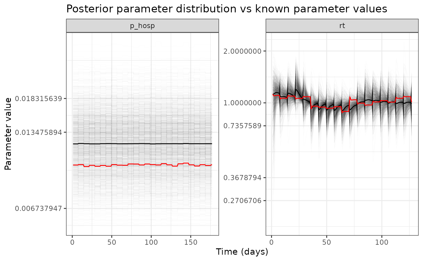
Get a dataframe of all of the key estimated model parameters combined with the key “known” model parameters to get a sense of which parameters we can recover and which might be unidentifiable (just as a first pass, eventually we will probably want to do a full sensitivity analysis to identify the regions of parameter space that are non-identifiable).

Note that if you are modifying this vignette to run on your own data skip this part– in the case of real data, we don’t know the true underlying model parameters.

static_params <- c(
  "eta_sd", "autoreg_rt",
  "autoreg_rt_site",
  "log_r_mu_intercept",
  "i0_over_n", "initial_growth",
  "inv_sqrt_phi_h", "sigma_ww_site_mean", "sigma_ww_site_sd",
  "p_hosp_mean", "p_hosp_w_sd", "t_peak", "viral_peak",
  "dur_shed", "log10_g", "ww_site_mod_sd",
  "infection_feedback"
)
vector_params <- c(
  "w", "p_hosp_w", "rt", "state_inf_per_capita", "p_hosp",
  "sigma_ww_site_raw", "ww_site_mod_raw",
  "ww_site_mod", "sigma_ww_site",
  "hosp_wday_effect"
)

matrix_params <- c("error_site")


# Get the full posterior parameter distribution from the real data
full_param_df <- get_full_param_distrib(
  all_draws, static_params, vector_params, matrix_params
)

# Compare to the knows parameters
param_df <- cfaforecastrenewalww::param_df # A set of the set static and dynamic
# from the `generate_simulated_data()` function default args. This is package data
comp_df <- full_param_df %>%
  left_join(param_df,
    by = c("name", "index_rows", "index_cols")
  )

ggplot(comp_df %>% filter(name %in% c("rt", "p_hosp"))) +
  geom_line(aes(x = index_cols, y = value, group = draw), size = 0.05, alpha = 0.05) +
  geom_line(aes(x = index_cols, y = median), color = "black") +
  geom_line(aes(x = index_cols, y = true_value), color = "red") +
  facet_wrap(~name, scales = "free") +
  theme_bw() +
  xlab("Time (days)") +
  ylab("Parameter value") +
  scale_y_continuous(trans = "log") +
  ggtitle("Posterior parameter distribution vs known parameter values")

ggplot(comp_df %>% filter(name %in% c("log10_g"))) +
  geom_histogram(aes(x = value), alpha = 0.3) +
  geom_vline(aes(xintercept = median), color = "black") +
  geom_vline(aes(xintercept = true_value), color = "red") +
  facet_wrap(~name, scales = "free") +
  xlab("Parameter value") +
  ylab("Frequency") +
  theme_bw() +
  scale_x_continuous(trans = "log") +
  ggtitle("Posterior parameter distribution vs known parameter values")

## `stat_bin()` using `bins = 30`. Pick better value with `binwidth`.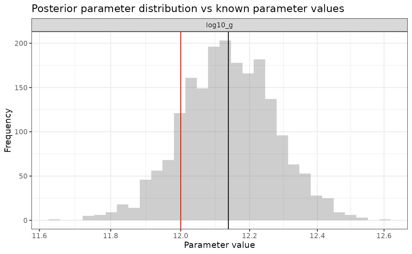

Try fitting the model without wastewater

The switch include_ww = 0 tells the model not to evaluate the likelihood on the wastewater data.

stan_data_hosp_only <- stan_data
stan_data_hosp_only$include_ww <- 0

fit_dynamic_rt_hosp_only <- model$sample(
  data = stan_data_hosp_only,
  seed = 123,
  init = init_fun,
  iter_sampling = 500,
  iter_warmup = 750,
  chains = 4,
  max_treedepth = 12,
  parallel_chains = 4
)

## Running MCMC with 4 parallel chains...
## 
## Chain 1 Iteration:    1 / 1250 [  0%]  (Warmup) 
## Chain 2 Iteration:    1 / 1250 [  0%]  (Warmup) 
## Chain 3 Iteration:    1 / 1250 [  0%]  (Warmup) 
## Chain 4 Iteration:    1 / 1250 [  0%]  (Warmup) 
## Chain 4 Iteration:  100 / 1250 [  8%]  (Warmup) 
## Chain 3 Iteration:  100 / 1250 [  8%]  (Warmup) 
## Chain 1 Iteration:  100 / 1250 [  8%]  (Warmup) 
## Chain 4 Iteration:  200 / 1250 [ 16%]  (Warmup) 
## Chain 2 Iteration:  100 / 1250 [  8%]  (Warmup) 
## Chain 1 Iteration:  200 / 1250 [ 16%]  (Warmup) 
## Chain 3 Iteration:  200 / 1250 [ 16%]  (Warmup) 
## Chain 4 Iteration:  300 / 1250 [ 24%]  (Warmup) 
## Chain 2 Iteration:  200 / 1250 [ 16%]  (Warmup) 
## Chain 1 Iteration:  300 / 1250 [ 24%]  (Warmup) 
## Chain 3 Iteration:  300 / 1250 [ 24%]  (Warmup) 
## Chain 4 Iteration:  400 / 1250 [ 32%]  (Warmup) 
## Chain 3 Iteration:  400 / 1250 [ 32%]  (Warmup) 
## Chain 1 Iteration:  400 / 1250 [ 32%]  (Warmup) 
## Chain 2 Iteration:  300 / 1250 [ 24%]  (Warmup) 
## Chain 4 Iteration:  500 / 1250 [ 40%]  (Warmup) 
## Chain 3 Iteration:  500 / 1250 [ 40%]  (Warmup) 
## Chain 1 Iteration:  500 / 1250 [ 40%]  (Warmup) 
## Chain 2 Iteration:  400 / 1250 [ 32%]  (Warmup) 
## Chain 4 Iteration:  600 / 1250 [ 48%]  (Warmup) 
## Chain 3 Iteration:  600 / 1250 [ 48%]  (Warmup) 
## Chain 1 Iteration:  600 / 1250 [ 48%]  (Warmup) 
## Chain 4 Iteration:  700 / 1250 [ 56%]  (Warmup) 
## Chain 2 Iteration:  500 / 1250 [ 40%]  (Warmup) 
## Chain 3 Iteration:  700 / 1250 [ 56%]  (Warmup) 
## Chain 1 Iteration:  700 / 1250 [ 56%]  (Warmup) 
## Chain 4 Iteration:  751 / 1250 [ 60%]  (Sampling) 
## Chain 2 Iteration:  600 / 1250 [ 48%]  (Warmup) 
## Chain 1 Iteration:  751 / 1250 [ 60%]  (Sampling) 
## Chain 3 Iteration:  751 / 1250 [ 60%]  (Sampling) 
## Chain 2 Iteration:  700 / 1250 [ 56%]  (Warmup) 
## Chain 4 Iteration:  850 / 1250 [ 68%]  (Sampling) 
## Chain 1 Iteration:  850 / 1250 [ 68%]  (Sampling) 
## Chain 2 Iteration:  751 / 1250 [ 60%]  (Sampling) 
## Chain 3 Iteration:  850 / 1250 [ 68%]  (Sampling) 
## Chain 1 Iteration:  950 / 1250 [ 76%]  (Sampling) 
## Chain 4 Iteration:  950 / 1250 [ 76%]  (Sampling) 
## Chain 1 Iteration: 1050 / 1250 [ 84%]  (Sampling) 
## Chain 2 Iteration:  850 / 1250 [ 68%]  (Sampling) 
## Chain 3 Iteration:  950 / 1250 [ 76%]  (Sampling) 
## Chain 4 Iteration: 1050 / 1250 [ 84%]  (Sampling) 
## Chain 1 Iteration: 1150 / 1250 [ 92%]  (Sampling) 
## Chain 1 Iteration: 1250 / 1250 [100%]  (Sampling) 
## Chain 1 finished in 102.8 seconds.
## Chain 2 Iteration:  950 / 1250 [ 76%]  (Sampling) 
## Chain 4 Iteration: 1150 / 1250 [ 92%]  (Sampling) 
## Chain 3 Iteration: 1050 / 1250 [ 84%]  (Sampling) 
## Chain 2 Iteration: 1050 / 1250 [ 84%]  (Sampling) 
## Chain 4 Iteration: 1250 / 1250 [100%]  (Sampling) 
## Chain 4 finished in 109.3 seconds.
## Chain 3 Iteration: 1150 / 1250 [ 92%]  (Sampling) 
## Chain 2 Iteration: 1150 / 1250 [ 92%]  (Sampling) 
## Chain 3 Iteration: 1250 / 1250 [100%]  (Sampling) 
## Chain 2 Iteration: 1250 / 1250 [100%]  (Sampling) 
## Chain 2 finished in 115.5 seconds.
## Chain 3 finished in 115.4 seconds.
## 
## All 4 chains finished successfully.
## Mean chain execution time: 110.8 seconds.
## Total execution time: 115.6 seconds.

all_draws_hosp_only <- fit_dynamic_rt_hosp_only$draws()

# Predicted observed hospital admissions
exp_obs_hosp <- all_draws_hosp_only %>%
  spread_draws(pred_hosp[t]) %>%
  select(pred_hosp, `.draw`, t) %>%
  rename(draw = `.draw`)
sampled_draws <- sample(1:max(exp_obs_hosp$draw), 100)


output_df_hosp_only <- exp_obs_hosp %>%
  left_join(
    train_data %>%
      select(
        date, t, daily_hosp_admits,
        daily_hosp_admits_for_eval
      ) %>%
      distinct(),
    by = c("t")
  ) %>%
  filter(draw %in% sampled_draws) # sample the draws for plotting

ggplot(output_df_hosp_only) +
  geom_line(aes(x = date, y = pred_hosp, group = draw),
    color = "red4", alpha = 0.1, size = 0.2
  ) +
  geom_point(aes(x = date, y = daily_hosp_admits_for_eval),
    shape = 21, color = "black", fill = "white"
  ) +
  geom_point(aes(x = date, y = daily_hosp_admits)) +
  geom_vline(aes(xintercept = forecast_date), linetype = "dashed") +
  xlab("") +
  ylab("Daily hospital admssions") +
  ggtitle("State level hospital admissions fit to only hospital admissions") +
  theme_bw()

## Warning: Removed 3700 rows containing missing values or values outside the scale range
## (`geom_point()`).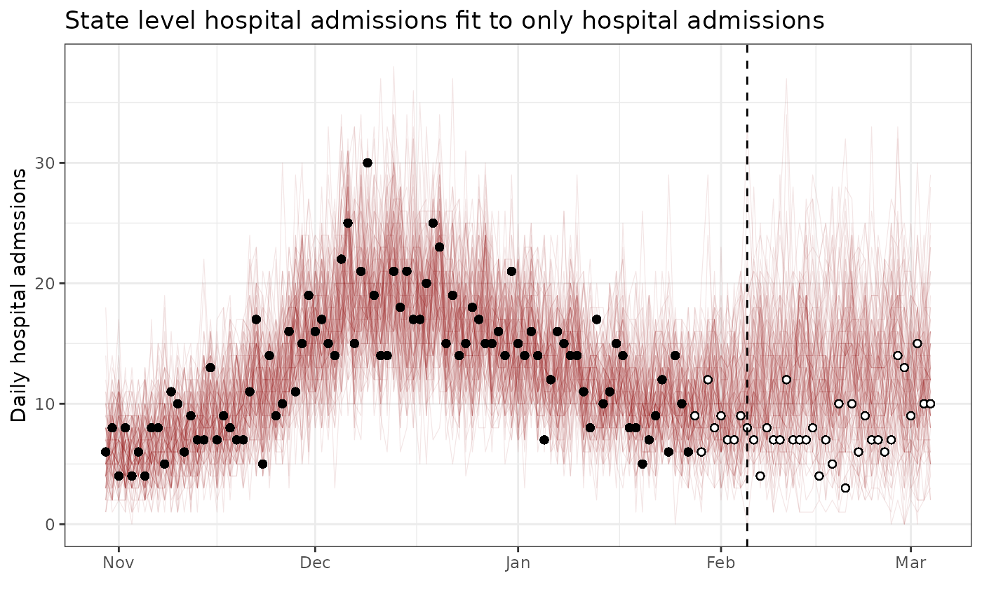

Model outputs: compare inferred parameters to known parameters

This time just for the IHR and R(t)

# Get the full posterior parameter distribution from the real data
full_param_df_hosp_only <- get_full_param_distrib(
  all_draws_hosp_only, static_params, vector_params, matrix_params
)

# Compare to the knows parameters
comp_df_hosp_only <- full_param_df_hosp_only %>%
  left_join(param_df,
    by = c("name", "index_rows", "index_cols")
  )

ggplot(comp_df_hosp_only %>% filter(name %in% c("rt", "p_hosp"))) +
  geom_line(aes(x = index_cols, y = value, group = draw), size = 0.05, alpha = 0.05) +
  geom_line(aes(x = index_cols, y = median), color = "black") +
  geom_line(aes(x = index_cols, y = true_value), color = "red") +
  facet_wrap(~name, scales = "free") +
  theme_bw() +
  xlab("Time (days)") +
  ylab("Parameter value") +
  scale_y_continuous(trans = "log") +
  ggtitle("Posterior parameter distribution vs known parameter values")

Kaitlyn Johnson

2023-12-20

Rationale

Load the data

Data exploration

Make some plots of the hospital admissions and wastewater data

Format data for inference in stan

Fit the wastewaster informed model

Look at the model outputs: generated quantities

Model outputs: compare inferred parameters to known parameters

Try fitting the model without wastewater

Model outputs: compare inferred parameters to known parameters