Low-level filtering
build_inference wraps a model in a ready-made engine (see Inference engines).
Underneath, ConfigurableEpi builds each piece of a state-space model separately, and those pieces can be wired into LowLevelParticleFilters.jl filters directly.
That gives access to per-step filtered states, smoothing and custom filters.
This example simulates data from a seasonal SEIRS model with a latent transmission modifier, then recovers the latent path with an unscented Kalman filter and smoother and with a bootstrap particle filter.
using ConfigurableEpi
using AlgebraicEpiMech
using Catlab: dom
using CairoMakie
using LinearAlgebra, Distributions, PositiveFactorizations
using LowLevelParticleFilters: UnscentedKalmanFilter, AdvancedParticleFilter, simulate,
    forward_trajectory, smooth, TrivialParams
import Random
Random.seed!(2026)
The model
An SEIRS model with the infectious compartment sampled into a two-stage observation chain.
The rate function receives the constrained latent drivers, the hyperparameters and model time in days; here transmission is a baseline \(R_0\) times a seasonal cosine times a latent modifier Rt that mean-reverts to 1.
N = 10_000.0
hyperparams = (gamma = 1.0, R0_baseline = 2.0, seasonal_amp = 0.15, N = N)

pn = attach_observation(dom(create_model(OnePopulationTyping(), SEIRS())), AtCompartment(:I); n_stages = 2)

function rates(latent, hyper, t)
    seasonal = 1.0 + hyper.seasonal_amp * cospi(2 * t / 365.0)
    return (transmission_S_I = hyper.gamma * hyper.R0_baseline * latent.Rt * seasonal / hyper.N,)
end
rate_defaults = (E_to_I = 0.5, I_to_R = 1.0, R_to_S = 1.0 / 180, obs_inflow_I = 1.0, O_I_1_to_O_I_2 = 0.5)
petri_vf! = build_petri_vf(pn, rates; defaults = rate_defaults)
Rt is an AR(1) latent (an Ornstein–Uhlenbeck process sampled each step) in the log chart of its init prior.
The StateLayout places compartments, observation accumulators and latents in one state vector, and build_stochastic_update turns the driver specs into the process-noise update.
latent_specs = (
    AR1ParamSpec(:Rt; init = positive_gaussian(:Rt, 1.0, 0.3), mu = 1.0, tau = 9.5, sigma = 0.34),
)
layout = StateLayout(pn, latent_specs; signal_names = (:reports,))
stochastic = build_stochastic_update(layout, latent_specs)
obs_model = (SignalObservationSpec(1, NegBinomialNoise(phi = 100.0); mean_modifier = 1.0, name = :reports),)
(ode_states = ode_names(layout), latents = layout.latent_names, dimension = layout.total_dim)
The observation uses the reset-accumulator pattern: at each step the last observation state is reset to zero and integrates that step's flow, which is read off directly as the expected count.
init = (S = N - 20.0, E = 10.0, I = 10.0, R = 0.0, O_I_1 = 0.0, O_I_2 = 0.0)
x0 = vcat([init[n] for n in ode_names(layout)], collect(stochastic.to_unconstrained((Rt = 1.0,))))
Unscented Kalman filter and smoother
build_full_dynamics gives one filter step (RK4 over supersample substeps of the day), and build_measurement_model the observation map.
Process noise enters only the latents and the accumulators, which build_R1 sizes.
dynamics = build_full_dynamics(petri_vf!, stochastic, layout; dt = 1.0, supersample = 4, obs_jitter = 1.0)
measure, n_obs, n_noise = build_measurement_model(layout, obs_model, stochastic)
R1 = Matrix(build_R1(layout))
R2 = Matrix{Float64}(I, n_noise, n_noise)
P0 = Matrix(Diagonal(vcat(fill(1.0e-6, length(ode_names(layout))), [0.2])))

ukf = UnscentedKalmanFilter{false, false, true, true}(
    dynamics, measure, R1, R2, MvNormal(x0, P0);
    p = hyperparams, ny = n_obs, nu = 0, weight_params = TrivialParams(),
    cholesky! = R -> cholesky!(Positive, Matrix(R)),
)
Simulate 40 days from the model itself, then filter and smooth.
T = 40
x_true, _, y_true = simulate(ukf, fill(Float64[], T), hyperparams)
y_data = [[round(max(y[1], 0.0))] for y in y_true]

sol = forward_trajectory(ukf, fill(Float64[], T), y_data)
sm = smooth(sol)
round(sol.ll; digits = 2)
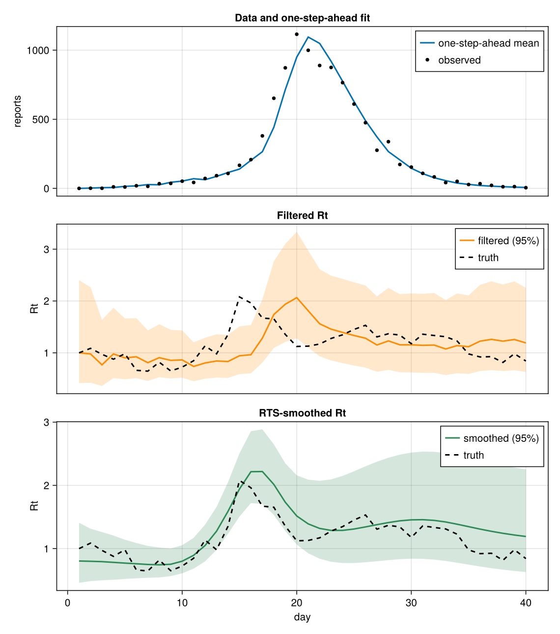
The latent lives in log space, so its 95% bands are pushed through exp.
The one-step-ahead predicted mean is the observation minus the innovation.
Rt(x) = stochastic.extract(x).Rt
li = layout.latent_range[1]
band(means, covs) = (
    [exp(means[t][li] - 1.96 * sqrt(max(covs[t][li, li], 0.0))) for t in 1:T],
    [exp(means[t][li] + 1.96 * sqrt(max(covs[t][li, li], 0.0))) for t in 1:T],
)
day, observed = 1:T, first.(y_data)
true_Rt, filt_Rt, smooth_Rt = Rt.(x_true), Rt.(sol.xt), Rt.(sm.xT)
filt_lo, filt_hi = band(sol.xt, sol.Rt)
smooth_lo, smooth_hi = band(sm.xT, sm.RT)

fig = Figure(size = (760, 860))
counts = Axis(fig[1, 1]; ylabel = "reports", title = "Data and one-step-ahead fit")
lines!(counts, day, observed .- first.(sol.e); label = "one-step-ahead mean", linewidth = 2)
scatter!(counts, day, observed; label = "observed", color = :black, markersize = 7)
axislegend(counts; position = :rt)

filtered = Axis(fig[2, 1]; ylabel = "Rt", title = "Filtered Rt")
band!(filtered, day, filt_lo, filt_hi; color = (:darkorange, 0.2))
lines!(filtered, day, filt_Rt; label = "filtered (95%)", linewidth = 2, color = :darkorange)
lines!(filtered, day, true_Rt; label = "truth", linewidth = 2, linestyle = :dash, color = :black)
axislegend(filtered; position = :rt)

smoothed = Axis(fig[3, 1]; xlabel = "day", ylabel = "Rt", title = "RTS-smoothed Rt")
band!(smoothed, day, smooth_lo, smooth_hi; color = (:seagreen, 0.2))
lines!(smoothed, day, smooth_Rt; label = "smoothed (95%)", linewidth = 2, color = :seagreen)
lines!(smoothed, day, true_Rt; label = "truth", linewidth = 2, linestyle = :dash, color = :black)
axislegend(smoothed; position = :rt)

linkxaxes!(counts, filtered, smoothed)
foreach(ax -> hidexdecorations!(ax; grid = false), (counts, filtered))
fig
Bootstrap particle filter
The same pieces adapt to a bootstrap particle filter.
Unlike the UKF's Gaussian innovations, the particle filter weights particles by the exact negative-binomial likelihood (build_measurement_logpdf) and simulates true count draws (build_pf_measurement).
The accumulator jitter is a UKF device, so it is off here.
pf_dynamics = build_pf_dynamics(
    build_full_dynamics(petri_vf!, stochastic, layout; dt = 1.0, supersample = 4, obs_jitter = 0.0), layout,
)
pf_measure = build_pf_measurement(layout, obs_model, stochastic)
loglik = build_measurement_logpdf(layout, obs_model, stochastic)

ode_var = (S = 4.0, E = 4.0, I = 4.0, R = 1.0, O_I_1 = 1.0, O_I_2 = 1.0)
P0_pf = Matrix(Diagonal(vcat([ode_var[n] for n in ode_names(layout)], [0.2])))
n_particles = 2_000
pf = AdvancedParticleFilter(
    n_particles, pf_dynamics, pf_measure, loglik, nothing, MvNormal(x0, P0_pf);
    p = hyperparams, ny = 1, nu = 0, rng = Random.Xoshiro(1),  # the filter's resampling RNG
)

T_pf = 60
x_pf, _, y_pf = simulate(pf, fill(Float64[], T_pf), hyperparams)
y_counts = [y[1:1] for y in y_pf]
sol_pf = forward_trajectory(pf, fill(Float64[], T_pf), y_counts)
round(sol_pf.ll; digits = 2)
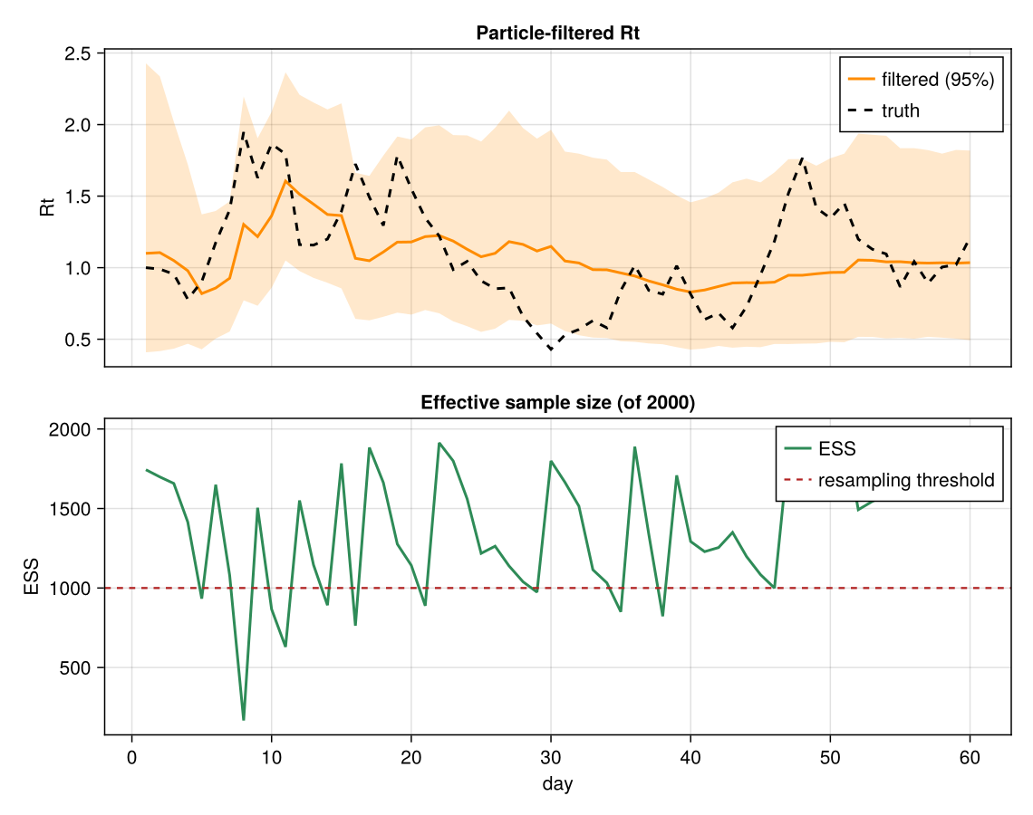
Summaries come from the weighted particle cloud: the weighted mean and 95% interval of Rt, and the effective sample size \(1 / \sum_i w_i^2\), which shows how often the cloud degenerates and is resampled.
function wquantile(vals, w, q)
    idx = sortperm(vals)
    cw = cumsum(w[idx]) ./ sum(w)
    return vals[idx][something(findfirst(>=(q), cw), length(vals))]
end

pf_Rt = zeros(T_pf); pf_lo = zeros(T_pf); pf_hi = zeros(T_pf)
for t in 1:T_pf
    rt, w = [exp(x[li]) for x in sol_pf.x[:, t]], sol_pf.we[:, t]
    pf_Rt[t], pf_lo[t], pf_hi[t] = sum(w .* rt), wquantile(rt, w, 0.025), wquantile(rt, w, 0.975)
end
ess = [1 / sum(abs2, sol_pf.we[:, t]) for t in 1:T_pf]

fig = Figure(size = (760, 600))
rt_panel = Axis(fig[1, 1]; ylabel = "Rt", title = "Particle-filtered Rt")
band!(rt_panel, 1:T_pf, pf_lo, pf_hi; color = (:darkorange, 0.2))
lines!(rt_panel, 1:T_pf, pf_Rt; label = "filtered (95%)", linewidth = 2, color = :darkorange)
lines!(rt_panel, 1:T_pf, Rt.(x_pf); label = "truth", linewidth = 2, linestyle = :dash, color = :black)
axislegend(rt_panel; position = :rt)

ess_panel = Axis(fig[2, 1]; xlabel = "day", ylabel = "ESS", title = "Effective sample size (of $n_particles)")
lines!(ess_panel, 1:T_pf, ess; label = "ESS", linewidth = 2, color = :seagreen)
hlines!(ess_panel, [n_particles / 2]; label = "resampling threshold", linestyle = :dash, color = :firebrick)
axislegend(ess_panel; position = :rt)

linkxaxes!(rt_panel, ess_panel)
hidexdecorations!(rt_panel; grid = false)
fig