Vignette 1: Calculate Cumulative Proximity for Geographic Areas
Sarah Rockhill
calc-proximity-to-hazards.RmdIntroduction
This vignette describes how the get_proximity() function
can be used to calculate cumulative proximity to select features for a
geographic area, such as a county, census tract, or neighborhood. The
get_proximity() function returns a vector of numeric values
representing cumulative proximity, or how close a community is to the
features of interest.
Cumulative proximity:
- Describes how near an area is to all features of interest, with higher values indicating that the area is generally closer to features than areas with lower proximity values.
- Is calculated by summing the inverse distances between the geometric center of each area and all features within a given search distance.
- Can be used to characterize potential population-level risk of exposure to environmental hazards.
- Can be weighted to account for the relative importance of each feature.
View hazprox datasets
In this example, we will calculate and analyze the cumulative
proximity to fires occurring in 2020 for census tracts in the state of
Georgia. A simple feature dataset representing all 2020 census tracts in
the State of Georgia is LazyLoaded with hazprox and can be
accessed directly as shown below. The Georgia census tracts,
ga, are provided as a sf MULTIPOLYGON object, allowing us
to perform geospatial analysis of these data directly. Viewing the
ga header reveals that the census tracts are projected in
NAD 1983 Georgia Statewide Lambert.
library(hazprox)
library(dplyr)
library(sf)
library(ggplot2)

#View first 5 census tract records
ga |> slice(1:5)
#> Simple feature collection with 5 features and 4 fields
#> Geometry type: MULTIPOLYGON
#> Dimension:     XY
#> Bounding box:  xmin: -210677.2 ymin: 11751900 xmax: 289688.3 ymax: 12254400
#> Projected CRS: NAD_1983_Georgia_Statewide_Lambert
#>   STATE       GEOID LSAD  POP                       geometry
#> 1    GA 13101880100   CT 1358 MULTIPOLYGON (((139670.9 11...
#> 2    GA 13271950500   CT 2897 MULTIPOLYGON (((123993.4 12...
#> 3    GA 13185011100   CT 3643 MULTIPOLYGON (((61964.23 11...
#> 4    GA 13277960700   CT 4639 MULTIPOLYGON (((-26934.43 1...
#> 5    GA 13095001500   CT 1803 MULTIPOLYGON (((-210579.6 1...
The hazprox package also includes a dataset with
information on 16,195 fires occurring in the state of Georgia from 2016
through 2020. The fires dataset is derived from the National Interagency
Fire Occurrence 6th Edition (1992-2020) dataset. These data are bundled
with the hazprox package as a comma separated values file
(ga_fires.csv) to demonstrate how to transform latitudinal
and longitudinal coordinates for analysis.
#Import fires dataset
fname <- system.file("extdata/ga_fires.csv", package = "hazprox")
ga_fires <- read.csv(fname)

#View first 5 records in the Georgia fires dataset
ga_fires |>
  select(Event, CauseType, Acres, Owner, Lat, Lon) |>
  slice(1:5)
#>                       Event CauseType Acres  Owner      Lat       Lon
#> 1   Recreation and ceremony     Human 22.00   USFS 34.75000 -83.77806
#> 2 Equipment and vehicle use     Human  0.10 COUNTY 34.63361 -85.05861
#> 3 Equipment and vehicle use     Human  1.00   USFS 33.38306 -83.41667
#> 4   Recreation and ceremony     Human  0.25   USFS 33.56028 -83.30667
#> 5   Recreation and ceremony     Human  0.10   USFS 33.03500 -83.72306
Each record in the ga_fires dataset includes latitude
(Lat) and longitude (Lon) coordinates representing the location for each
fire origin. We will need to convert these records into spatial points
before calculating proximity. You can use the help()
function to view metadata for datasets bundled with hazprox. The
metadata includes important information about each dataset, including
its source, field descriptions, and processing steps that were performed
during dataset preparation.
help("ga_fires")The ga_fires documentation indicates that the geographic
coordinates are in North American Datum of 1983 (NAD 83). We can use the
sf library to convert these data to a points simple feature.
Prepare data for analysis
For this demonstration, because we are only interested in fires
occurring during 2020, we will filter the fires_sf dataset
based on the Year column.
fires_sf <- fires_sf |> filter(Year == 2020)The fires_sf dataset contains a column for the total
number of acres burned (Acres). We can use this information to weight
each fire by severity. First, let’s examine the distribution of acres
burned.
summary(fires_sf$Acres)
#>    Min. 1st Qu.  Median    Mean 3rd Qu.    Max.
#>   0.010   0.200   0.750   3.421   2.675 309.400
The number of acres burned shows a highly right-skewed distribution. Most fires burn fewer than 7 acres of land; however, the largest fire burned over 300 acres. For this analysis, we will exclude fires less than one acre and create a weight based on the number of acres burned. Due to the skewed distribution, we will log-transform acres.
Visualize fires
Let’s take a look at where fires are located throughout Georgia by plotting the fire coordinates on a map of Georgia. We will vary the size and color of each point by the weight we calculated in the previous step to highlight where the most severe fires were located.
fires_sf |>
  arrange(Severity) |>
  ggplot() +
  geom_sf(data = ga, color = NA, fill = "gray40") +
  geom_sf(aes(size = Severity, color = Severity), alpha = 0.5) +
  scale_color_distiller(palette = "Spectral",
                        limits = c(0, 6),
                        breaks = seq(0, 6, by = 2),
                        guide = 'legend') +
  scale_size_continuous(range = c(2, 10),
                        limits = c(0, 6),
                        breaks = seq(0, 6, by = 2)) +
  labs(title = "Fires (1+ Acres) Occuring in Georgia, 2020") +
  theme_minimal()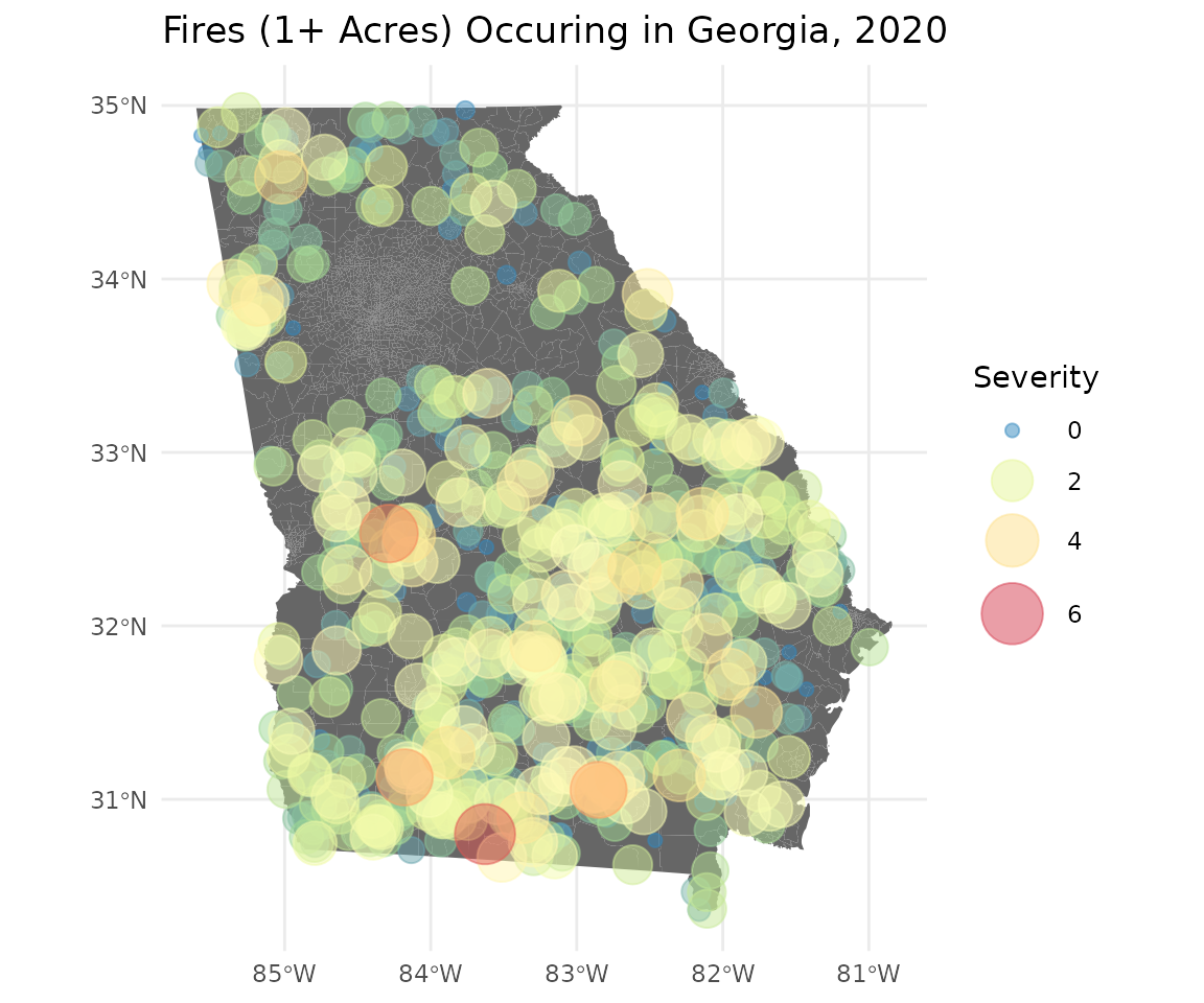
Fires are dispersed throughout most the state, with the exception of the Atlanta metro area. The largest fires appear to be clustered within the southwestern quadrant of the state.
Calculate proximity
Next, let’s examine how the cumulative proximity is distributed
across census tracts in the state using the get_proximity()
function. We will weight each fire by the log of the total acres burned
(severity). We can also exclude fires occurring more than 25 km from
each block group boundary by setting the tolerance to 25. Note, other
units of length can be used to specify the tolerance by providing a
“units” argument (e.g., units = ‘mi’).
Although we previously converted our fires data to spatial data with an associated geographic coordinate reference system, these data are not currently projected. Typically, we want both our polygon features and our hazards to have the same projected coordinate reference system (CRS), but let’s see what happens if we neglect to project one of our inputs.
wts <- fires_sf$Severity
ga$Proximity <- get_proximity(ga, fires_sf, tolerance = 25, weights = wts)
#> to does not have a projected CRS.
#> Projecting to into (+proj=lcc +lat_0=0 +lon_0=-83.5 +lat_1=31.4166666666667 +lat_2=34.2833333333333 +x_0=0 +y_0=0 +datum=NAD83 +units=us-ft +no_defs).
When we apply get_proximity() to the unprojected fire
locations, we get the following warning message:
to is not in a projected CRS.

Projecting to into (+proj=lcc +lat_0=0 +lon_0=-83.5 +lat_1=31.4166666666667 +lat_2=34.2833333333333 +x_0=0 +y_0=0 +datum=NAD83 +units=us-ft +no_defs).
This message informs us that because fires_sf lacks a projection, the
get_proximity function has projected it for us using the
same CRS as the from layer (ga). Note, this message does
not indicate an error. The function will succeed when only one of the
input datasets is not projected because it assumes that the unprojected
data should have the same CRS as the other input. However, if neither
input has a projected CRS or if they have a different CRS,
get_proximity will return an error.
Descriptive statistics
Now let’s examine the distribution of the proximity value by requesting a histogram.
ggplot(ga, aes(Proximity)) +
  geom_histogram(fill = "navy", color = "white") +
  ggtitle('Distribution of Census Tract Proximity to 2020 Fires')+
  ylab('Census Tracts (n)') +
  theme_minimal()
#> `stat_bin()` using `bins = 30`. Pick better value `binwidth`.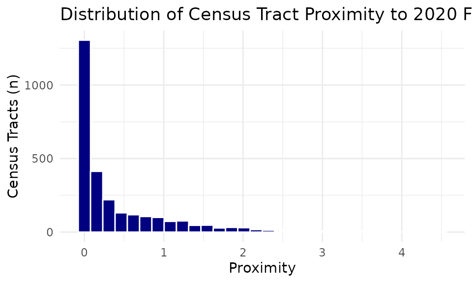
Most tracts have relatively low proximity. The median score is 0.104. However, a few tracts have very high proximity scores.
View map of proximity
We can use ggplot2 to visualize the geographic
distribution of census tracts across Georgia by proximity score.
ga |>
  ggplot(aes(fill = Proximity)) +
  geom_sf(color = NA) +
  scale_fill_distiller(palette = "Spectral") +
  labs(title = "Census Tract Proximity to Fires Burning 1+ Acre",
       subtitle = "Georgia, 2020") +
  theme_minimal()
The choropleth map above highlights census tracts with greater
overall proximity to fires burning more than one acre in 2020. This map
appears to agree with the overall trend displayed in the point-level
map, but it provides more visual clarity and reveals tracts outside the
southwest quadrant with high proximity. This concludes the
get_proximity vignette; however, users may consider
additional applications of cumulative proximity statistics to public
health issues. For example, proximity scores can be used to identify
communities or facilities with the most potential for exposure to
various environmental health risks. Proximity scores can be used to
target health education and outreach or used to model relationships
between population-level exposure burden and health outcomes.